

1 Introduction
Plankton communities typically display spatio–temporal scale-dependent irregular oscillations. Such complex dynamics can be explained by random fluctuations in the surrounding environment. An alternative view is that at least part of the apparent disorder is due to deterministic chaos. Although chaotic dynamics appears to be rather common on models of ecological dynamics [1], convincing evidence for chaos in natural ecological systems remain meager [1,2]. There are many reasons for this, including noise in ecological data, and impracticality of experimental manipulation of ecological systems. Nevertheless, a great deal of interest is focused on the possibility of using conceptual (minimal) mathematical models to describe, explain and give possible scenarios of biological population dynamics.
Conceptual models are proved to be an appropriate tool for searching and understanding basic mechanisms of plankton spatio–temporal dynamics. Their usefulness has been demonstrated in the studies of plankton patchiness and phytoplankton blooms [3–8]. Recently, the effects of external hydrodynamical forcing in the appearance of non-equilibrium spatio–temporal plankton patterns have been studied [9,10]. Conceptual models have also been applied to investigate the plankton pattern formation resulting from planktivorous fish school walks without any hydrodynamical forcing [11–13]. Predator–prey limit cycle oscillations, plankton front propagation, and the generation and drift of plankton patches were found in a minimal phytoplankton–zooplankton interaction model [14,15] that was originally formulated by Scheffer [16]. The emergence of diffusion-induced chaos has been found by Pascual [17] along a linear nutrient gradient in the same model without fish predation.
In this paper we focus on the chaotic dynamics of plankton communities in the patchy marine environment where not only transient spatial patterns but also more stable structures associated with ocean fronts [18] and cyclonic rings [19,20] exist. We compare the dynamics of the plankton communities with and without the time delay T1 associated with a zooplankton maturation period [21] (in literature, other causes of delays in population dynamics at various time scales are also considered [22,23]). The main result of this paper is that the time delay can lead to progressively replacing regular plankton dynamics by chaos.
2 Models
We consider two modifications of the 1D basic marine food chain model [16]:
- (1) at T1=0, the dynamics of phytoplankton P(X,τ) and zooplankton H(X,τ) population at any point X and time τ are given by the following differential equations:
(1) (2) - (2) at T1≠0, differential equation (2) transforms into the integrodifferential equation
(3)
The model can be simplified by introducing dimensionless variables. Following Pascual [17], we introduce p=P/K and h=AH/K. Space is scaled by the size of the numerical mesh L/k, where L is the total length of the considered area and k+1 is the number of nodes of the mesh. Thus, L/k is the scale of the expected spatial processes. Time is scaled by a characteristic value of the phytoplankton growth rate R0. As a result, x=kX/L, and t=R0τ. Eqs. (1)–(3) become:
| (4) |
| (5) |
| (6) |
In this paper, we assume that the inhomogeneity of the environment only affects the fish population, i.e. the fish predation rate f=f(x), whereas all other parameters are constant. For the sake of simplicity, we assume that f is equal to a certain constant value in the fish-populated patches, otherwise f=0.
The diffusion terms in Eqs. (4)–(6) often describe the spatial mixing of the species due to the self-motion of the organisms [24]. However, in natural waters, it is turbulent diffusion that is supposed to dominate plankton mixing [25]. Taking this into account, we consider both phytoplankton and zooplankton as passive contaminants of the water turbulent motion. In this case, dp=dh=d. Using the relationship between turbulent diffusivity and the scale of the phenomenon in the sea [25] with the minimum phytoplankton growth rate R0 given by 10−6 s−1 [26], the characteristic length L/k of about 2 km typical of plankton patterns, one can show that d is about 5×10⁻². It should be noted that since our goal is to investigate plankton patterns on kilometer scales, we do not consider the behavior of plankters at the individual level.
For numerical integration of Eqs. (4)–(6), a simple explicit difference scheme is used [27]. The 1D space is divided into a grid of 64 finite-difference cells of unit length. The border between habitats divides the space into two patches.
The time step is set as equal to 10−2. Repetition of the integration with smaller step sizes showed that the numerical results did not change, ensuring the accuracy of the chosen steps. The plankton dynamics is investigated with no-flux boundary conditions. The initial distributions for p and h are uniform and the same for both habitats.
3 Plankton dynamics in homogeneously distributed communities
Fig. 1 demonstrates the zooplankton solution diagrams for systems 4, 5 (where the time delay associated with a zooplankton maturation period is absent) and 4, 6 (where T≠0). In other words, Fig. 1 shows the dependence of steady-state solutions (at d=0) on the fish predation rate f for three values of the time delay; namely, for T1=0, and also for rather common values of T1 [21]: 30 days and 50 days (corresponding values of T in Eq. (6) are equal to 2.6 and 4.3). Appropriate solution diagrams for phytoplankton are not shown here because of a strong interdependence between phytoplankton and zooplankton dynamics. Many early observers have already reported that there is an inverse relationship between phytoplankton and zooplankton, i.e. phytoplankton density is lower when zooplankton density is higher, and vice versa. Such an inverse relationship is an apparent consequence of phytoplankton grazing by zooplankton [3].
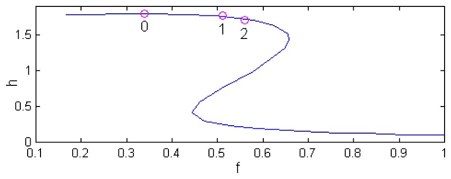
h-solution diagrams of the model (4), (5) and the model (4), (6) for the following set of parameters [27]: r=5, a=5, b=5, m=0.6, n=0.4. This set of parameters is used throughout the work. Point 0 denotes the Hopf bifurcation at T=0 while points 1 and 2 mark Hopf bifurcations at T=2.6 and T=4.3, correspondingly.
One can see that the zooplankton low-density stationary states (which the phytoplankton-dominated stationary states correspond to) are typical of high predation rates f. When lowering f, an unstable and another stable steady state appear, which make the system bistable. Further lowering of f, the bistability disappears in a saddle-node bifurcation. For some value of f (Fig. 1, T=0), the Hopf bifurcation occurs (point 0), destabilizing the zooplankton-dominated steady state while creating a stable limit cycle. When increasing T, the Hopf bifurcation shifts into the bistability region (Fig. 1, point 1 for T=2.6 and point 2 for T=4.3). In these cases, the region of oscillatory plankton dynamics becomes wider. Notice that the equilibrium points (p0,h0) of Eqs. (4) and (5) remain equilibrium points in the presence of the lag (Eqs. (4) and (6)). Indeed, the only term that Eq. (6) differs from Eq. (5) is . At the point (p0,h0) this term becomes ap0h0/(1+bp0) that coincides with the corresponding term in Eq. (5). Hence, at this point, ∂h/∂t (Eq. (5))=∂h/∂t (Eq. (6))=0.
4 Spatial plankton patterns in a two-habitat system
Let us consider the simplest example of a spatially structured ecosystem consisting of two habitats. The dynamics in both the habitats obeys Eqs. (4) and (5) at T=0, or Eqs. (4) and (6) for T≠0. In one of the habitats f=0, i.e. fish is absent (for example due to local changes in temperature or salinity [31,32]). The diffusion interaction between these habitats leads to plankton spatial pattern formation even at T=0 [27,32]. Note that the interaction between the habitats is essential to disturb the initially homogeneous spatial plankton distribution. Otherwise, no patterns could occur.
In order to demonstrate the dependence of the plankton spatial patterns on the fish predation rate f and the lag T in detail, we construct pattern bifurcation diagrams. Fig. 2 shows the zooplankton abundance as a function of position x (the horizontal axis) calculated at t=2500 for different values of f and for four values of T from T=0 to T=4.5. The spatial distributions of the model phytoplankton abundance (not shown) are in an inverse relationship with the zooplankton distributions [27]. One can see that at T=0, the structures with larger inner scale characteristics for the smaller f transform into small-scale irregular patterns as f grows. The following growth of the fish predation rate leads (in the fish-populated habitat) to the nearly homogeneous high-level zooplankton abundance as the local dynamics of the system passes through the Hopf bifurcation (cf. Fig. 1, point 0), and to the low-level zooplankton abundance as soon as the local dynamics reaches the low-density stationary states. In contrast, in the fish-free habitat, the Hopf bifurcation is not accompanied by essential changes in the plankton spatial structure (Fig. 2, T=0). The expansion of the region with oscillatory dynamics observed in the solution diagrams as the time lag T becomes nonzero and grows (Fig. 1) is accompanied by shrinking (along f-direction) of the region of the large-scale patterns and broadening of the irregular small-scale region. Besides, in contrast to the irregular plankton distributions typical of the fish-free habitat at relatively small values of T the ordered (nearly periodical) spatial plankton patterns emerge in the fish-free habitat at high fish predation rate values (Fig. 2 at T=3.5 and T=4.5) that characterize phytoplankton-dominated stationary states (Fig. 1).
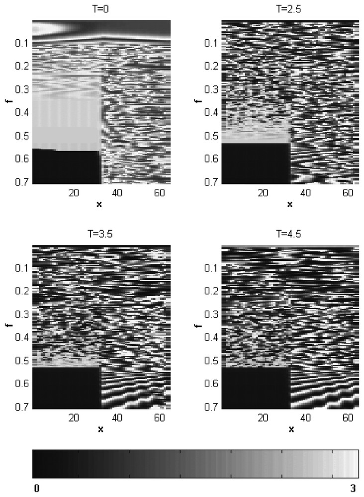
Pattern bifurcation diagrams for zooplankton obtained for T=0, T=2.5, T=3.5 and T=4.5 (shown above each of the pattern bifurcation diagrams) after 250 000 iterations; x is the spatial coordinate; f is the fish predation rate. The zooplankton density scale is given in the lover part of the figure.
5 Temporal plankton dynamics in the two-habitat system
To study temporal changes in the plankton abundance, we use values and , i.e. the length of the vectors characterizing phytoplankton and zooplankton density distributions in each of the habitats:
| (7) |
| (8) |
Fig. 3 enables us to compare the -dynamics with and without the time lag that is due to zooplankton maturation (the sophisticated treatment of the spatio–temporal plankton dynamics at T=0 has been carried out in the work [27]). One can see that at T=0 (the left column), two attractors can coexist: the limit cycle (for which values of dominant Lyapunov exponent λ are around zero), and the chaotic attractor (for which λ>0). As a result, small changes in starting conditions (for example, in the h0 values; p0 is set constant) can lead to both regular oscillations of the plankton abundant and the chaotic plankton dynamics (segments of the corresponding time series are shown above each of the functions λ(h0) of Fig. 3). Interestingly, for the system with T=0, there is a large region of the initial zooplankton densities for which the basin of attraction to the limit cycle is intertwined in a complicated way with the basin of the chaotic attractor [27].
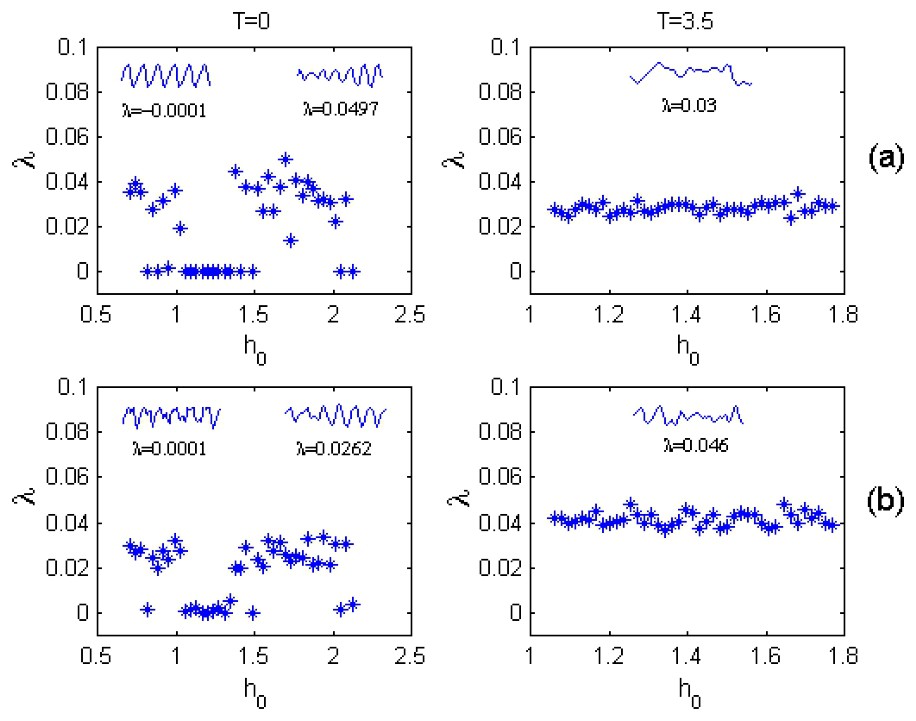
Dominant Lyapunov exponents λ for various initial zooplankton densities h0 under T=0 (left column) and T=3.5 (right column) calculated for the fish-populated (a) and fish-free (b) habitats; p0=0.35; f=0.18. Segments of regular (when λ is around zero) and chaotic time series and corresponding values of the dominant Lyapunov exponent are shown above each of the functions λ(h0).
At T≠0 the plankton dynamics changes drastically. The limit cycle disappears, and the only chaotic attractor (for which λ>0) is found to influence the plankton dynamics in both the fish-free and fish-populated habitats (the right column of Fig. 3). Notice that variations of the dominant Lyapunov exponent are obviously less pronounced in the case of the time-delay dynamics in comparison with those at T=0. The correlation between the λ variations in the fish-populated and fish-free habitats are also evident (cf. Fig. 3(a) and (b)).
It is notable that in contrast to the case when T=0, at T≠0 chaotic dynamics can occur even at small values of the fish predation rate, if only the time delay T is more than a critical value Tcr. As an example, Fig. 4 shows such a transition from regular to chaotic plankton dynamics at f=0.05 as T passes the critical value (Tcr=2.25).
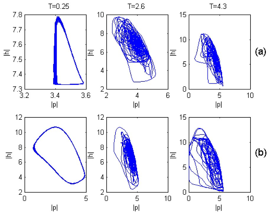
Plankton dynamics in both (a) fish-populated and (b) fish free habitats under different values of T.
6 Discussion
Plankton communities often show large fluctuations both in zooplankton and algal biomass. Such irregular patterns can be explained by inaccurate sampling or by stochastic environmental effects on the population. At the same time, irregularity in plankton dynamics can be due to the chaotic rather than stochastic nature of the processes that underlie spatio–temporal changes in the plankton abundance. Indeed, the results of the analysis of field data [28] indicate that the recorded dynamics of diatom communities can be chaotic. Our results show that both irregularity in plankton spatial distributions (Fig. 2) and chaoticity of plankton temporal oscillations (Fig. 3) can be affected by the time lag due to zooplankton maturation.
The length of the time delay can be critical for chaos development. Short lags do not lead to chaotic plankton dynamics at small values of the fish predation rate (Fig. 4). The critical values Tcr obtained in our simulations are smaller than the values of maturation period of zooplankton that have been obtained in the course of field observations [21]. This implies that chaotic dynamics is an inherent feature of aquatic ecosystems. Indeed, there is increasing evidence that the systems with chaotic dynamics have an even higher potential for adapting to changing environmental conditions than the systems with regular behavior [29,30]. In view of this, studying interrelations between chaotic and regular regimes of population dynamics should be significant.
Acknowledgements
We are grateful to unknown referees for their comments, and also to Drs R. Aliev and A. Morozov for fruitful discussions. This research was supported by DFG, NSF and RFBR grants, and by the University of California Agricultural Experiment Station.