

Abbreviations
SSE:
secondary-structure element
3D:three dimension
lu:lattice unit
MC:Monte Carlo cycle
TH:topohydrophobic
Cα:alpha carbon
PMF:potential of mean force
MJ:Miyazawa and Jernigan
1 Introduction
Protein folding is a major challenge at the period of complete genome determination, and we are now in the post genomic era. Many of the attempts for ab initio prediction of protein tertiary structures go through the prediction of regular secondary structures, helices and strands. Two approaches have been developed at both short and long time limits. Molecular dynamics allow investigating either small deviations in 3D structures due for instance to local mutations, or small proteins, but is limited until now to short timescales, up to 1 μs [1]. Large timescales can be reached with simplified models, such as Monte Carlo simulations in discrete spaces. Starting from a random coil conformation, the folding process can be dynamically simulated. It has already been demonstrated [2] that multi-fragment intermediate states are observed. A fragment is a certain number of successive residues that collapse and form a local compact structure, linked to another one by an extended polypeptide chain. These fragments are correlated with secondary-structure elements (SSE) as it has already been shown, by using a simple cubic lattice [3]. In this paper, we focus exclusively on the first steps of the folding process and try to delineate the fragments formed at this stage. The time limits have been chosen in a way that the number of fragments is maximal, before the folding process reaches a single compact domain. We demonstrate here a correspondence between fragments and SSE on a set of 42 proteins, representative of various folds. The physical reason for this correspondence may be based on the fact that local interactions (from the point of view of the sequence) play a key role in the formation of SSE, but also probably constitute the major driving force of folding. To carry out this project, a 24-first-neighbour lattice [4] has been used, in order to give a better flexibility to the macromolecular chain and to have a better approximation of real protein angles, particularly for β strands. We have performed calculations utilising two different potentials of mean force (PMF) to describe the interactions between pairs of residues: the classical Miyazawa–Jernigan (MJ) potential [5,6] and a new one, based on the concept of ‘topohydrophobic’ residues, i.e. positions always occupied by a hydrophobic residue for all the members of a common fold [7,8]. Starting from 100 initial conformations for every protein, we have recorded the residues included in each fragment, and performed a statistical analysis over the protein set. The quality factor estimating the one-residue correspondence between SSE, as derived by DSSP [9] and fragments, gives an overall mean value of 61%. Moreover, regions separating fragments are mainly occupied by loops in the 3D structures of the proteins. Fragments also reasonably fit (mean quality factor of 67%) the hydrophobic clusters deduced from the HCA method [10,11]. The role of hydrophobic residues is important as they mainly contribute to the driving force of fragment formation. This study shows that regular local structures may be formed at the very first steps of the folding. These observations are otherwise consistent with the features of a folding of proteins by blocks, i.e. fragments of around 27 residues, that have been called TEF (for Tightened End Fragments) as their ends are mainly occupied by topohydrophobic residues located in close contacts, i.e. at less than 7 Å [12].
2 Methods
2.1 Lattice geometry
A protein is represented as a self-avoiding chain, composed of the Cα atoms only. We have used a lattice, introduced by Skolnick et al. [4] where the Cα are located on the nodes of an underlying simple cubic lattice and positioned in the following way: consecutive Cα atoms are separated by a vector of the form (2,1,0). The length of this vector, corresponding to the mean distance between Cα in proteins, is set to 3.8 Å or 51/2 lattice units (lu). This lattice unit corresponds to the underlying simple cubic lattice, and is worth 1.7 Å [4]. Each Cα in this (2,1,0) lattice can have 24 first neighbours. Since the occupied volume of amino acids must be taken into account, we make the assumption that two amino acids (contiguous or not) may not be closer than 3.8 Å. To approximate protein chain geometry, we have limited the angle between three contiguous Cα, thus limiting the local flexibility. This is done by restricting the distance between residues i and i+2 from 4.1 to 7.2 Å (or from 61/2 to 181/2 lu), corresponding to angles from 66° to 143° respectively [4], in better agreement with real angles in alpha and beta conformations.
2.2 Energy of interaction
In this model, the amino acid type is not introduced in the chain geometry (which considers only Cα), but is taken into account in the energy terms, which describe the inter-residue non-covalent interactions. We assume that two non-contiguous residues with a distance smaller than 7.2 Å (181/2 lu) interact with an energy that depends on their nature. Outside this limit, their interaction energy is zero. The selected interaction range exceeds the minimal allowed distance between neighbour Cα atoms, which is 3.8 Å. Therefore, it accounts much better for the environment of each residue than a simple cubic-lattice model with nearest-neighbour interactions.
Two expressions of the pair interacting residue energy have been used in this study. The first one was the distance-independent statistical pair potential of Miyazawa and Jernigan [5,6], which constitutes a 20×20 symmetric matrix. This potential implicitly takes into account the solvent effect (the hydrophobic interaction).
We derived another potential of mean force (PMF), called topohydrophobic (TH) from a database of 340 structurally aligned proteins [8] of various folds. It takes into account the fact that some positions in the multiple alignment of a family are always occupied by strong hydrophobic residues, that is V, I, L, M, F, Y, W. These positions have been called topohydrophobic [7,8] and it has been shown that they are related to the folding nucleus [13–15]. Thus, in a protein, there are two possible states for the above seven hydrophobic residue types: topohydrophobic or not. The remaining 13 residue types exist only in the non-topohydrophobic state. Therefore three matrices have been built. The first one is a 20×20 matrix, which defines the energy of interaction between non-topohydrophobic residues, named NN for non-topohydrophobic–non-topohydrophobic. The second is a 7×20 matrix, which describes the interaction between a topohydrophobic and a non-topohydrophobic residue, named TN for tophohydrophobic–non-topohydrophobic. The third one is a 7×7 matrix, describing the interactions between residues in topohydrophobic positions, named TT for topohydrophobic–topohydrophobic. To derive these matrices, we used the procedure described by Bryant and Lawrence [16], which deals with log-linear modelling from the number of contacts between different types of amino acids in a dataset. The data for such an analysis takes the form of a four-dimensional contingency table, whose category variables are the two amino acid types r and s, the distance interval of contacts d, and the protein p. The cells contain the ratio of the observed contacts Nrsdpobs between residues r and s at distance d over Nrsdpexp, the expected number of contacts by mass action or random pairing [16]. Assuming a Boltzmann-like distribution of contacts is equivalent to considering that the frequency of occurrence of a particular contact is proportional to exp(−ΔE/RT). These energy differences ΔE may be viewed as chemical potentials μ as in Eq. (1):
| (1) |
| (2) |
The method of iterative fitting was used to find the maximum likelihood estimates of these parameters, and extrapolate their values independently of the protein p, such that μrs≈μrsp [16]. The parameters μrs constitute the energy of interaction between two residues in the three matrices, NN, TN and TT.
2.3 Monte Carlo folding algorithm
The initial state of the proteins is an extended random conformation. At each step, a single residue is selected at random to move and its move is also chosen at random and follows the previous lattice restrictions. The single residue movements are of two kinds: end flip movement for the N and C terminal residues and corner movements for the others. All the possible corner moves are described in detail in the paper of Skolnick and co-workers [4]. These authors also use multiple-residue moves and a more sophisticated representation of proteins by introducing side chains in order to simulate formation and conservation of secondary structures. Here, our goal is to reveal the role of local interactions (in the sense of sequence) at the first stages of folding and to show that they guide the protein into intermediate multi-fragment states. This is why we restricted the move set in the elementary single residue moves, which are sufficient to drive the protein into a fragmented state.
After each move, the energy is calculated for the new state and is accepted with a probability:
| (3) |
2.4 Definition of a fragment
A fragment is a piece of sequence that folds to form a compact geometry in the first stages of the folding process simulated by our Monte Carlo algorithm. At that time, the protein is composed of a set of fragments, linked by coil-like parts of the sequence (Fig. 1).
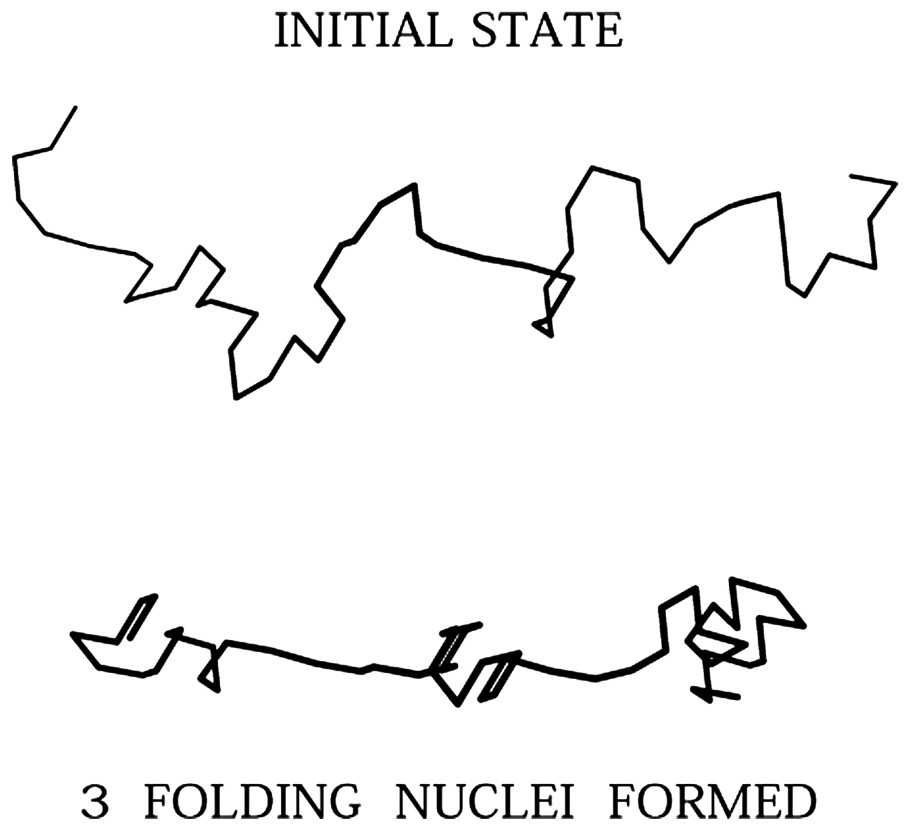
Initial and intermediate state, as an example of fragment formation during the Monte Carlo simulated folding. The initial state is chosen at random but as extended as possible. The intermediate state is composed of three fragments.
During a simulation, a residue belongs to a fragment if it is part of a set of at least four non-contiguous residues interacting by pairs. Actually there are at least six pairs of interacting residues in the smallest fragment. By interacting we mean that the distance of each pair is equal or less than 7.2 Å or 181/2 lu, the maximum range of non-covalent interactions.
The number of fragments decreases with time, as they progressively merge to form fewer and longer ones until the protein forms a single globule. We are interested to find the highest possible number of fragments with the highest lifetime. Thus the time interval must satisfy two requirements. First, the length and composition of the fragments should not be dependent on the initial state and second the time interval must be sufficiently large to allow a statistical analysis on the fluctuations of the limits. The first requirement determines the low time limit tmin and the second the high time limit tmax, and time is measured in Monte Carlo (MC) steps in our case. In addition to that, we must take into account that, due to the serial nature of the algorithm, the time limits are correlated to the protein chain length L. We have determined that for small proteins of about 50 residues, tmin is around 105 MC and . Thus, we have adopted the following linear relation to generalise tmin and tmax to proteins of any length:
| (4) |
| (5) |
In order to avoid any effect due to the initial conformation, 100 extended initial states have been generated at random for each protein. For each of the 100 simulations per protein, the number and limits of fragments are recorded every 100 MC between tmin and tmax, giving a total number of recorded states of the order of 104. It thus enables us to decide for any residue if it belongs or not to a fragment. For the ith simulation over 100 for a given protein, n(i,f) is the number of recorded intermediate states containing f fragments. From the maximum No(i) of the distribution of n(i,f), typically 104, one deduces the number of fragments f∘(i). In other words, for each one of the 100 simulations, we select the fragmentation that corresponds to the longest lifetime. To accurately calculate the limits of the fragments, we count the number of times occ(i,r) each residue r is included in a fragment over all the No(i) states. By defining ocm(i) as the maximum value of occ(i,r) over all residues, we assume that any residue such that occ(i,r)>0.9ocm(i) belongs to a fragment. This is equivalent to averaging over the time period in which the number of fragments remains constant, in order to decide if a given residue is involved or not in a fragment. By this mean, we determined the limits of the f∘(i) fragments for the ith simulation. This procedure is repeated for all the 100 initial conformations. We then construct a new histogram OCC(r) that represents the number of times a residue r belongs to a fragment over the 100 simulations. The maximum value of OCC(r) is 100, thus the final fragmentation is obtained by assuming that residue r belongs to a fragment if OCC(r) is larger than a limit which depends on the potential used, 50 for TH and 65 for MJ.
2.5 Protein set
A set of 42 proteins has been selected from the PDB [17] corresponding to the main characteristic folds, and they are given in Table 1. Secondary-structure assignments have been computed by DSSP [9]. All these proteins have been simulated with the MJ field. A subset of 22 of the above proteins, for which the topohydrophobic residues are known, has been studied also with the TH field.
Description of fragments obtained from Monte Carlo simulation in a set of 42 proteins of various folds, using the Jernigan and Miyazawa potential. The PDB code is given in the first column. The PDB codes followed by an asterisk indicate the presence of at least one disulfide bridge in the protein. The classification from CATH [32] is also given. QS and QH are one-residue quality factors (see methods) with respect to DSSP assignment and HCA prediction. F is the number of fragments determined by the present method and C is the number of clusters deduced from HCA. N is the number of SSE as derived from DSSP. F is compared to both N and C by means of global quality factors Quality factors RS and RH range from 0 to 1 and describe the match between F versus N and C respectively. A good correspondence between fragments and SSE occurs when both QS and RS have high values. Mean quality factor values are given for each of the four CATH classes, namely a (mainly alpha), b (mainly beta), ab (alpha and beta) and f (few secondary structures)
| PDB code | CATH | QS (%) | QH (%) | F | C | N | RS (%) | RH (%) |
| 3c2c | a | 62 | 63 | 6 | 7 | 5 | 80 | 86 |
| 2mhr | a | 60 | 72 | 6 | 9 | 6 | 100 | 67 |
| 1hbg | a | 84 | 83 | 7 | 8 | 7 | 100 | 88 |
| 2lhb | a | 64 | 77 | 8 | 12 | 9 | 89 | 67 |
| 1bp2∗ | a | 60 | 60 | 7 | 7 | 9 | 78 | 100 |
| 1eca | a | 68 | 75 | 9 | 8 | 8 | 88 | 88 |
| 1enh | a | 67 | 63 | 5 | 4 | 3 | 33 | 75 |
| 1rro | a | 73 | 64 | 7 | 9 | 11 | 64 | 78 |
| 4cpv | a | 75 | 73 | 6 | 8 | 8 | 75 | 75 |
| 155 c | a | 54 | 65 | 8 | 8 | 6 | 67 | 100 |
| 2mhb | a | 67 | 74 | 7 | 10 | 7 | 100 | 70 |
| 1ibe | a | 65 | 73 | 8 | 9 | 7 | 86 | 89 |
| 1dke | a | 72 | 74 | 8 | 10 | 7 | 86 | 80 |
| 1lsg∗ | a | 61 | 72 | 7 | 10 | 10 | 70 | 70 |
| 3cyt | a | 47 | 61 | 6 | 8 | 5 | 80 | 75 |
| 1utg | a | 63 | 79 | 4 | 5 | 5 | 80 | 80 |
| 1ag2∗ | a | 61 | 70 | 5 | 7 | 5 | 100 | 71 |
| Class a mean | 65 | 70 | 81 | 80 | ||||
| 1pk4∗ | b | 37 | 61 | 4 | 4 | 4 | 100 | 100 |
| 1tud | b | 67 | 68 | 3 | 6 | 6 | 50 | 50 |
| 1pmy | b | 65 | 69 | 9 | 10 | 10 | 90 | 90 |
| 1fas∗ | b | 49 | 43 | 4 | 4 | 5 | 80 | 100 |
| 2mcm∗ | b | 59 | 59 | 6 | 8 | 10 | 60 | 75 |
| 4rxn | b | 50 | 67 | 3 | 5 | 6 | 50 | 60 |
| 1rei∗ | b | 53 | 64 | 5 | 9 | 11 | 45 | 56 |
| 2sns | b | 62 | 69 | 10 | 9 | 12 | 83 | 89 |
| 1qab | b | 59 | 67 | 8 | 9 | 10 | 80 | 89 |
| 2tpi∗ | b | 59 | 67 | 13 | 15 | 17 | 76 | 87 |
| 1pwt | b | 66 | 70 | 4 | 6 | 6 | 67 | 67 |
| Class b mean | 57 | 64 | 71 | 78 | ||||
| 1bdm | ab | 65 | 75 | 6 | 8 | 7 | 86 | 75 |
| 1frd | ab | 53 | 60 | 7 | 8 | 11 | 64 | 88 |
| 1fxd∗ | ab | 53 | 53 | 3 | 6 | 6 | 50 | 50 |
| 1ptf | ab | 67 | 75 | 5 | 6 | 7 | 71 | 83 |
| 1sha | ab | 66 | 76 | 8 | 10 | 8 | 100 | 80 |
| 3chy | ab | 62 | 73 | 8 | 9 | 10 | 80 | 89 |
| 5p21 | ab | 71 | 78 | 12 | 11 | 12 | 100 | 91 |
| 1dur | ab | 50 | 52 | 4 | 3 | 5 | 80 | 67 |
| 1cyo | ab | 62 | 75 | 5 | 5 | 10 | 50 | 100 |
| 1c0b∗ | ab | 67 | 62 | 6 | 6 | 9 | 67 | 100 |
| 5nll | ab | 73 | 68 | 11 | 9 | 12 | 92 | 78 |
| Class ab mean | 63 | 68 | 76 | 82 | ||||
| 1isu | f | 50 | 56 | 4 | 4 | 4 | 100 | 100 |
| 1knt∗ | f | 55 | 51 | 3 | 3 | 4 | 75 | 100 |
| 1hip | f | 44 | 58 | 4 | 4 | 8 | 50 | 100 |
| Class f mean | 50 | 55 | 75 | 100 | ||||
| Total mean | 61 | 67 | 77 | 81 |
2.6 Validation of fragment prediction: comparison with DSSP SSE assignments and HCA clusters
The calculated fragments have been compared to SSE assigned by the DSSP algorithm [9]. Another comparison has been performed with the results of the HCA method. HCA lies on a threading of the residues along an alpha helix, followed by a projection in a 2D plane. In this representation, neighbouring hydrophobic residues constitute clusters [10,11]. One cluster is built of hydrophobic residues separated by at most three non-hydrophobic ones and at the condition that no proline is present, because proline is considered as a cluster breaker. It has been shown that there is an agreement between HCA clusters and SSE [18]. HCA clusters have been compared to the derived fragments, except for clusters formed of a single residue.
2.7 Quantitative analysis
Agreement between the number of fragments and the number of SSE has been calculated with a one-residue quality factor, QS. It is derived from the classical Q3 quality factor used in SSE prediction papers [19], in order to differentiate alpha helices, beta strands and coiled structures. In our case, the amino acids fall into two categories: either they belong to a SSE or not, whatever the nature of the SSE (alpha or beta), because the fragments do not provide information on the type of secondary structure. If p is the number of amino acids belonging both to a fragment and to a SSE and n the number of those not belonging to a fragment and a SSE, the quality factor is defined as:
| (6) |
| (7) |
The maxima of RS and RH are 1, which correspond to N=F or N=C. An equivalent factor RH has been computed to compare F to the number C of HCA clusters.
3 Results
For all the 42 proteins typical of various folds from the PDB studied in this lattice model, the simulated folding process went through the formation of intermediate states, composed of compact fragments linked by pieces of sequence in non-compact conformations. The number of fragments decreases with time until a final globular state is reached. During its lifetime, the 3D internal geometry of a fragment changes, but its linear limits are surprisingly stable. This characteristic property led us to compare amino acid compositions of fragments and SSE. In order to accurately determine the most stable fragmentation for each protein, we performed a statistical analysis of the recorded states in a predetermined time range at the beginning of folding, presented in detail in the Methods section. The results concerning fragment formation are presented in Table 1 for a 42-protein set, calculated with the MJ potential. Table 2 shows the results of the same calculations with the TH potential. They concern 22 proteins, a subset of the total 42 proteins, where the topohydrophobic positions are known and permit the use of TH field.
Description of fragments obtained from Monte Carlo simulation in a subset of 22 proteins included in the dataset of Table 1. The TH mean potential described in this work has been used. Notations are identical to those of Table 1
| PDB code | CATH | QS (%) | QH (%) | F | C | N | RS (%) | RH (%) |
| 3c2c | a | 64 | 52 | 6 | 7 | 5 | 80 | 86 |
| 2mhr | a | 52 | 64 | 6 | 9 | 6 | 100 | 67 |
| 1hbg | a | 73 | 67 | 10 | 8 | 7 | 57 | 75 |
| 2lhb | a | 59 | 61 | 8 | 12 | 9 | 89 | 67 |
| 1bp2∗ | a | 52 | 67 | 7 | 7 | 9 | 78 | 100 |
| 1eca | a | 67 | 76 | 8 | 8 | 8 | 100 | 100 |
| 1enh | a | 63 | 56 | 3 | 4 | 3 | 100 | 75 |
| 1rro | a | 69 | 69 | 5 | 9 | 11 | 45 | 56 |
| Class a mean | 62 | 64 | 81 | 78 | ||||
| 1pk | b | 47 | 58 | 3 | 4 | 4 | 75 | 75 |
| 1tud | b | 68 | 60 | 3 | 6 | 6 | 50 | 50 |
| 1pmy | b | 64 | 57 | 6 | 10 | 10 | 60 | 60 |
| 1fas∗ | b | 54 | 41 | 3 | 4 | 5 | 60 | 75 |
| 2mcm | b | 57 | 46 | 7 | 8 | 10 | 70 | 88 |
| Class b mean | 58 | 52 | 63 | 70 | ||||
| 1bdm | ab | 57 | 67 | 7 | 8 | 7 | 100 | 88 |
| 1frd | ab | 56 | 69 | 7 | 8 | 11 | 64 | 88 |
| 1fxd∗ | ab | 57 | 53 | 3 | 6 | 6 | 50 | 50 |
| 1ptf | ab | 60 | 63 | 5 | 6 | 7 | 71 | 83 |
| 1sha | ab | 52 | 58 | 5 | 10 | 8 | 63 | 50 |
| 3chy | ab | 62 | 62 | 7 | 9 | 10 | 70 | 78 |
| 5p21 | ab | 65 | 67 | 8 | 11 | 12 | 67 | 73 |
| Class ab mean | 58 | 63 | 69 | 73 | ||||
| 1isu | f | 61 | 61 | 4 | 4 | 4 | 100 | 100 |
| 1knt∗ | f | 47 | 44 | 3 | 3 | 4 | 75 | 100 |
| Class f mean | 54 | 53 | 88 | 100 | ||||
| Total mean | 59 | 60 | 74 | 76 |
With the MJ potential, the one-residue correspondence QS reaches a maximum of 84% for hemoglobin (PDB code 1hbg) (Table 1). QS values are very sensitive to the class of fold. Class a proteins, corresponding to mainly alpha in CATH, give rise to the highest values, with a mean at 65%. It is followed by the ab class (alpha–beta) with a mean at 63%, and by the b class (mainly beta) with a mean at 57%. Last is the f class (few SSE) with a mean at 50%. In most cases, the number of SSE is higher than the number of predicted fragments. The quality factor, RS, is 1 in a few cases, and its class dependence follows the one-residue quality factor QS, with mean values of 81% for class a, 76% for class ab and 71% for class b, while it is 75% for class f. The one-residue quality factor for hydrophobic clusters, QH, also follows the same class dependence. The mean value of QH is 70% for class a, 68% for class ab, 64% for class b and 55% for class f. The quality factor RH is nearly class-independent, being 80% for class a, 82% for class ab, 78% for class b, while it is worth 100% for class f. These results indicate a close relationship between fragments and hydrophobic clusters.
With the TH potential, the maximum of QS on the 22-protein subset also occurs for hemoglobin (1hbg) at 73% (Table 2). The mean value of QS is less class dependent: it is 62% for class a, 58% for classes ab and b. RS is much higher for class a (81%), than for classes ab and b (69% and 63% respectively). QH is clearly better for classes a and ab (64% and 63% respectively) than for class b (52%). RH has the same class dependence as RS, being 78% for class a, versus 73% and 70% for classes ab and b, respectively. The class f has been skipped from our statistical analysis because it only comprises two elements.
To better understand these results, Fig. 2 represents the histograms OCC(r) (see Methods) showing the number of times each residue is involved in a fragment over 100 Monte Carlo runs corresponding to 100 different initial states. These histograms provide the final fragmentation for a selection of four proteins (1hbg, 2mcm, 1bdm, 1isu), one from each CATH class, with both MJ (broken line) and TH (solid line) potentials. One important feature is the high conservation of the limits of the fragments, whatever initial state the simulation starts from. This permits a clear determination of the limits of the fragments by using an appropriate cut-off for each potential. We actually use cut-off values of 65% for MJ potential and 50% for TH potential. The second feature is that, despite the different physical nature of the two potentials, their results are similar for most of the predicted fragments. In the case of 1hbg (mainly alpha) 7 SSE are assigned by DSSP, while the MJ potential predicts seven fragments and the TH 10. RS and RH are 100% and 88% for MJ, while they are worth 57% and 75% for TH potential. The TH potential builds two minor peaks, which result in two new fragments: one in between SSE1 and SSE2, and the second one inside SSE5. Moreover, SSE6 corresponds to one fragment with MJ potential, while it is split into two with the TH potential, with a minimum between them close to zero, so that the new fragmentation is not due to any cut-off effect. SSE6 is a long helix, which contains four topohydrophobic positions located in the N-terminal part. This might be the reason why this long helix is split into two fragments precisely at the position of the last topohydrophobic residue. Besides, in the loop between SSE6 and SSE7, there is a methionine, which will be included in the new fragment. With 2mcm (mainly beta), DSSP assigns 10 SSE. TH potential still predicts more fragments than MJ (7 versus 6), but both RS and RH are better for TH in this case, because the number of predicted fragments with TH is closer to the actual number of assigned SSE. The TH potential predicts a second fragment shorter than MJ and better describes the loop in between SSE2 and SSE3. Fragment 4 from MJ has been split into two new fragments with TH and the inter-fragment region corresponds to the loop in between SSE6 and SSE7. Thus the separations performed by the TH potential better account for the actual number of SSE in this case. If one looks at fragment 3 by TH potential, it corresponds to two strands, and the cut-off value of 50% is too low to separate them. For 1bdm (alpha beta class) the number of fragments is increased by one with TH potential. In the case of 1isu (few SSE class), there are four fragments in each case of potential. The TH potential slightly better fits the SSE1, and there are two topohydrophobic residues at the end of cluster 1 (top of Fig. 2d), which do not belong to SSE1. As these two amino acids are second neighbours along the sequence, they produce a constant effect on the potential, as they are permanently in interaction. The fragment will be forced to form by the presence of the hydrophobic residues located towards the N terminal. A common consideration about Fig. 2 and the difference between both potentials is the fact that TH always produces more pronounced separations between fragments.
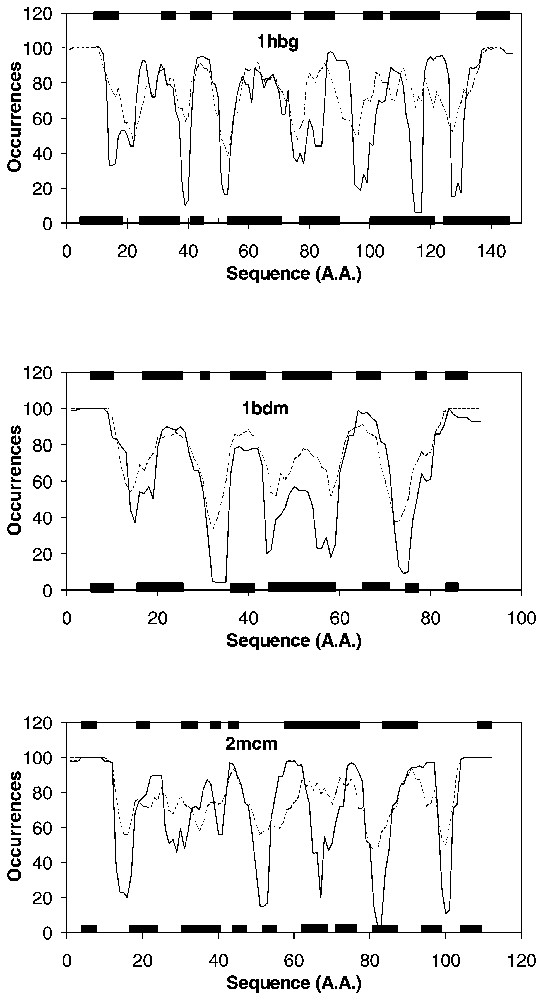
Histograms of the fragments derived with both potentials used in this study, on four examples: 1hbg (alpha class), 2mcm (beta class), 1bdm (alpha beta class) and 1isu (few class). They are constructed by summing up the presence of a residue in a fragment for 100 initial states. Below each curve are represented the various SSE assigned by DSSP, and on the top the clusters from HCA. Solid lines: TH potential, broken lines: MJ potential.
To better visualise the correspondence between SSE and fragments, the same four examples of proteins are represented in Fig. 3 with the 3D structures and the pieces of sequences corresponding to the predicted fragments are coloured in green when TH potential was used and in blue for the MJ potential. For haemoglobin (1hbg), with the TH potential, most of the long helices belong to a fragment. The last two parallel helices correspond to three fragments, with the central one, which contains the turn linking the two helices. For the MJ potential, these two helices correspond to two fragments, but the loop in between them is included in the first fragment. In the case of 1bdm, malate dehydrogenase, the TH potential misses one turn of the helix, which is alone to face the sheet. This helix will be included, as well as the last strand, in a fragment with the MJ potential. For 2mcm, beta turns are mainly included in one single fragment, as well as some longer loops, for both potentials. The only difference between the two potentials occurs for b5, which belongs to a fragment only for TH. With 1isu, the SSE are fairly small, and they are all included in fragments, whatever the potential, the only difference being that the first fragment of MJ is clearly longer that with TH.
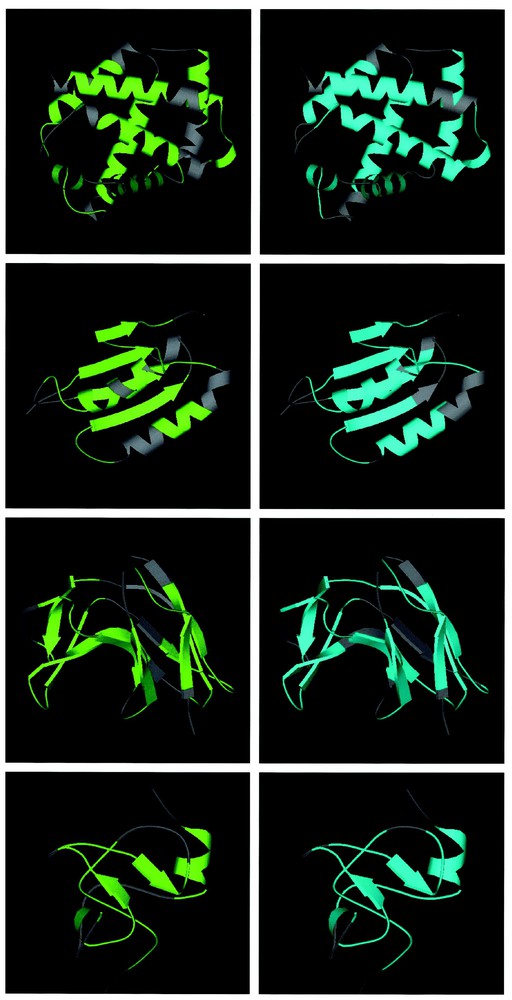
3D structures of the same proteins as in Fig. 2 represented with MOLSCRIPT [33]. All proteins have been coloured such that all inter-fragment regions are in grey, fragments derived from the TH potential are in green (left), and fragments derived from the MJ potential are in blue (right). From top to bottom: 1hbg (class a), 1bdm (class ab), 2mcm (class b) and 1isu (class f).
4 Discussion
A simulation of protein folding on a discrete space has been performed. A (2,1,0) lattice has been used, which permits to reasonably approximate the backbone geometry of real proteins. Two different potentials of mean force have been used, the classical one from Miyazawa and Jernigan, and a new one that includes the particular behaviour of hydrophobic residues highly conserved at a given position through evolution. It is a clear improvement relative to simple cubic lattice, especially in its ability to reproduce the geometry of beta strands. During this folding simulation, before one compact globular state is reached, the protein is formed by a succession of compact fragments whose limits in sequence are stable over time. Our approach is restricted to the early steps of folding and is focused on the analysis of the fragments formed during this period. Care has been taken to select the time range for which the maximum number of fragments occurs, provided they have a sufficient lifetime. This is an extension of our previous work [3] where it was established that fragments are very much sequence-dependent and correspond to one or several elements of secondary structures. Here we present results on a set of 42 proteins of various folds where we particularly investigated the correlation between SSE and fragments. For this purpose, a one residue quality factor QS has been calculated to quantify the agreement between the states to which a residue is assigned. It is based on the classical quality factor Q3 used for testing secondary-structure predictions [20], but restricted in our case to a two-state prediction. There is a clear correspondence between calculated fragments and SSE, as it can be seen from the QS overall mean value (around 60% for both potentials). This is corroborated by the matching between the numbers of fragments and SSE, giving a mean value of RS around 78%.
A QS factor of 60% is quite low from the point of view of prediction, but this was not our goal. By running these simulations, we aimed at elucidating how and to what extent the information on secondary structures is introduced since the beginning of the folding process, guiding thus rapidly the protein towards the tertiary structure. Our model simulates essentially the role of local interactions, in the sense of sequence. The formation of fragments in the SSE regions demonstrates that an important part of the sequence-structure code is contained in these local interactions. We expect that long-range interactions are necessary to stabilise the tertiary structure and adjust the limits of SSE. The number of fragments is often smaller than the number of SSE, but a common feature, as can be seen in the four histograms of fragment positions plotted in Fig. 2, is that most of the inter fragment regions fall into loops, i.e. regions connecting regular SSE [21,22]. Thus fragments mainly correspond to one or several SSE, with a clear preference for a single SSE.
From a dynamical point of view, our simulations provide insights to the folding mechanism. During their lifetime, multiple fragment intermediate states are not structurally stable, but they are stable in terms of sequence. Their conformation does not freeze, which would be an obstacle to rapid folding. Our approach could conciliate the framework model of folding and the nucleation condensation approach: on one hand, hierarchic folding seems to occur since compact fragments are observed, and on the other hand, their conformation is dynamically changing. Once a nucleation fragment is formed, it remains fairly constant in sequence, during approximately one order of magnitude of timescale, before a new state with fewer fragments appears, and so on until a single globule is formed. From an analysis of the Φ-values of six small proteins, Nölting and Andert [23] conclude that proteins (at least small ones) “proceed by means of formation of clusters of residues neighboured in the 3D structure which are particularly rich in residues that belong to regular secondary structures.” These authors reconcile the nucleation-condensation mechanism (due to a non-uniform distribution of the structural consolidation) with the framework model (consolidation is higher at positions of SSE) for folding in a generalized nucleation condensation. The main transition state is composed of a few clusters of residues on average more included in SSE than the rest of the molecule. Thus our approach is compatible with the one of Nölting and Andert. Our results are also consistent with the work of Baldwin and Rose [24,25], who simulated the initial steps of folding and showed that the tendency of residues to take their native secondary-structure conformation exists at the beginning of folding and is due to local interactions.
Global quality factors, illustrating the agreement between the numbers of predicted fragments and assigned SSE, are similar whatever potential is employed. As the number of fragments is roughly potential-independent, this implies that the algorithm is robust towards this number of compact fragments. The MJ potential seems to be sensitive to the class of proteins and produces the best correspondence in the case of alpha helices, i.e., in cases where the local interactions, in terms of sequence, are predominant even in the native state. The TH potential is also class-sensitive, maybe in a lesser extent: the values of QS are nearly class-independent, but the agreement between numbers of fragments and SSE, reflected by the RS factor has the same class dependence as for MJ, giving the higher values for mainly alpha proteins. These remarks are coherent with the fact that in vivo helices are generally formed at a timescale smaller than strands, due precisely to the predominance of local interactions at the beginning of the process [24,25]. We noticed that in general proteins with disulfide bridges have low QS values, as indicated in Tables 1 and 2. The presence of disulfide bridges, especially for small proteins, is one limitation of our model in its present state. One might try to overcome this point, by splitting in the PMF the two contributions of free cysteins and half cystins, linked through a covalent disulfide bridge. Free cysteins actually behave like hydrophobic residues, in particular for the buried character, while cystins do not [26].
There is a clear correspondence between predicted fragments and hydrophobic clusters derived from HCA, revealed by the values of both QH and RH factors. In this study, we compared a Monte Carlo simulation to the HCA data because this latter has been proven to be a useful tool in the determination of precise SSE using only information from the sequence. HCA is based on a physicochemical background, i.e., the phase separation of protein structures into hydrophobic core and hydrophilic envelope. The clear observed similarity between these two conceptually different methods lies on the fact that they basically consider local interactions along the macromolecular chain, which produce a local aggregation of hydrophobic residues. The fragments described in this paper can be related to the concept of building blocks used in the literature [27–29]. The building blocks are defined as compact units with a hydrophobic core and they are composed either of a single secondary structure or of a contiguous segment consisting of interacting structural elements in the work by Tsai et al. [28]. In this latter case, the building blocks can be combined to form hydrophobic folding units. Their building block is a contiguous sequence fragment with a variable size, and it is a highly populated transient structure. We do believe that the presently observed fragments correspond to the non-overlapping building blocks of Tsai et al. and we focus our analysis on a timescale such that it leaves constant the size of the fragment. Their approach needs to have the structure of the protein, and is thus an assignment, while we are interested in the prediction aspect. One can also relate our fragments to the notion of foldons, used in a prediction process by Gilis and Rooman in the early steps of folding [30], but they are slightly longer, as they are constituted of several consecutive SSE.
The principals underlying the method developed in the present paper are consistent with the notion of closed loops introduced by Berezovsky and Trifonov [31], which are fragments of preferred length around 27 amino acids. These closed loops, recently called TEF for Tightened End Fragments [12] are such that on average both ends are close in the 3D structures, and occupied by topohydrophobic residues. The correspondence between these proto fragments and the TEF must be further investigated.
Acknowledgements
We would like to thank the financial support of the European Union through the contract QLG2-CT-2002–01298 and the French–Greek bilateral cooperation Plato for Grant No. 04146WM.