

1 Introduction
Jatropha curcas L. (Euphorbiaceae) is a perennial small tree or large shrub that is distributed across semiarid tropical and subtropical regions of the Americas, Africa, and Asia [1,2]. J. curcas is a monoecious plant with unisexual flowers and has a high rate of self-pollination [3]. J. curcas has wide adaptability to a range of ecological habitats and climatic conditions and high potential for greening and eco-rehabilitation of wastelands [3]. J. curcas has recently become popular due to its potential economic value, as it has a relatively high content of seed oil, which can be used as biodiesel [4].
The geographic center of origin of J. curcas remains controversial. Botanists have hypothesized that J. curcas was distributed by Portuguese seafarers from Central America, via Cape Verde to Africa and Asia [3]. The plant has been widely disseminated and has become naturalized in many tropical and subtropical regions. Its current geographical distribution is vague and insufficient for recovering genetic structure due to the interference of forces like domestication and potential genotype- environment interactions [5]. A better understanding of the geographic origin, genetic structure, intraspecific relatedness, and differentiation among J. curcas germplasms would provide insights into population structure, breeding programs, and conservation of genetic resources. Molecular approaches are powerful for tracking geographic origins and introduction histories of exotic species, reconstructing evolutionary relationships, and assessing genetic variation in the colonization process [6].
Previous studies on the genetic variation in J. curcas germplasms have been conducted using various types of molecular markers such as AFLPs [7,8], ISSRs [9], RAPDs [10], and SSRs [11]. These studies demonstrated that genetic variation in Central America is much higher than that in other regions [12–14]. However, few studies have reported the genetic variation and structure of J. curcas on all continents simultaneously. The internal transcribed spacer region (ITS1-5.8S-ITS2) of nuclear ribosomal DNA (nrDNA) is one of the most popular and effective genetic markers for the inference of phylogenetic relationships and evolutionary studies in plants [15].
In the present study, we sampled 102 accessions of J. curcas from 11 countries that are representative of the plant's distribution across Asia, Africa, and the Americas. Using ITS sequencing, we had the following aims:
- • evaluate the genetic variation and genetic diversity level within accessions and among haplotypes;
- • determine phylogenetic relationships and estimate genetic divergence of J. curcas accessions;
- • explore the center of origin of J. curcas and its potential dispersal route.
2 Materials and methods
2.1 Plant materials
A total of 102 accessions of J. curcas were collected from the following 11 countries: 72 from China, 7 from India, 7 from Vietnam, 5 from Burma, 4 from Thailand, 2 from Indonesia, 1 from Laos, 1 from Zambia, 1 from Burkina Faso, 1 from Mali, and 1 from Brazil. The accessions from China are highly representative of within-country dispersal, with 69 accessions collected from 6 provinces in southwestern and southern China, including 3 hybrid varieties. These materials were kindly provided by the Tropical Eco-Agriculture Institute of the Yunnan Academy of Agricultural Sciences and Institute of Tropical Bioscience and Biotechnology, CATAS. The ITS spacer region of 102 J. curcas accessions were sequenced in this study, and 20 additional sequences (from plants in India, Madagascar, Cape Verde, Spain, Brazil, and Mexico) were obtained from GenBank (National Center for Biotechnology Information; NCBI). The sample code, location, latitude, longitude, altitude, country, haplotype, and GenBank accession number of all accessions are listed in Table 1. Jatropha gossypifolia was used as an outgroup for phylogenetic analysis [1].
List of Jatropha curcas L. samples used in the present study with sample code, locality, latitude, longitude, altitude, country, individual haplotype and GenBank accession number. Jatropha gossypifolia was used as an outgroup.
| Sample code | Locality | Latitude (N) | Longitude (E) | Altitude (m) | Country | HP | GenBank Accession |
| Jatropha curcas | |||||||
| CHGZ1 | Leyuan, Guizhou | 25°11’36.60” | 105°54’22.39” | 417 | China | H1 | KP190940 |
| CHGZ2 | Lekang, Guizhou | 25°03’15.32” | 106°13’33.44” | 412 | China | H1 | KP190941 |
| CHGZ3 | Zhenfeng, Guizhou | 26°47’38.47” | 102°00’04.53” | 1079 | China | H4 | KP190942 |
| CHGZ4 | Ceheng, Guizhou | 24°54’50.99” | 105°35’40.54” | 560 | China | H5 | KP190943 |
| CHGD | Zhanjiang, Guangdong | 21°14’50.10” | 110°10’20.15” | 10 | China | H1 | KP190944 |
| CHH1 | Sanya, Hainan | 18°29’10.00” | 109°43’42.87” | 45 | China | H1 | KP190945 |
| CHH2 | Sanya, Hainan | 18°29’10.00” | 109°43’42.87” | 45 | China | H1 | KP190946 |
| CHH3 | Sanya, Hainan | 18°29’10.00” | 109°43’42.87” | 45 | China | H1 | KP190947 |
| CHH4 | Sanya, Hainan | 18°29’10.00” | 109°43’42.87” | 45 | China | H1 | KP190948 |
| CHH5 | Sanya, Hainan | 18°29’10.00” | 109°43’42.87” | 45 | China | H1 | KP190949 |
| CHH6 | Sanya, Hainan | 18°29’10.00” | 109°43’42.87” | 45 | China | H1 | KP190950 |
| CHH7 | Qiongshan, Hainan | 19°12’20.05” | 109°31’10.00” | 120 | China | H1 | KP190951 |
| CHH8 | Hainan | - | - | - | China | H1 | KP190952 |
| CHH9 | Hainan | - | - | - | China | H1 | KP190953 |
| CHH10 | Changjiang, Hainan | 19°04’16.00” | 109°02’40.55” | 118 | China | H3 | KP190954 |
| CHH11 | Dongfang, Hainan | 19°03’43.01” | 108°30’06.53” | 67 | China | H1 | KP190955 |
| CHH12 | Haikou, Hainan | 19°32’38.41” | 110°10’53.85” | 93 | China | H6 | KP190956 |
| CHH13 | Jianfengling, Hainan | 18°26’25.15” | 108°27’46.58” | 70 | China | H3 | KP190957 |
| CHH14 | Qiongzhong, Hainan | 19°05’00.13” | 109°29’18.20” | 195 | China | H1 | KP190958 |
| CHS1 | Lazha, Sichuan | 26°21’41.08” | 101°55’25.48” | 985 | China | H7 | KP190959 |
| CHS2 | Tongde, Sichuan | 26°42’26.26” | 101°33’26.89” | 1349 | China | H1 | KP190960 |
| CHS3 | Miyi, Sichuan | 26°53’22.77” | 102°05’51.47” | 1115 | China | H1 | KP190961 |
| CHS4 | Lazha, Sichuan | 26°22’15.53” | 101°55’42.08” | 960 | China | H8 | KP191042 |
| CHS5 | Yanyuan, Sichuan | 27°42’38.96” | 101°57’49.29” | 1409 | China | H1 | KP190962 |
| CHS6 | Yanyuan, Sichuan | 25°50’38.97” | 101°49’54.30” | 1093 | China | H1 | KP190963 |
| CHS7 | Yanyuan, Sichuan | 27°42’33.03” | 101°58’12.58” | 1300 | China | H1 | KP190964 |
| CHS8 | Dechang, Sichuan | 26°34’54.65” | 101°43’07.67” | 1148 | China | H1 | KP190965 |
| CHS9 | Huili, Sichuan | 26°12’53.16” | 102°07’33.53” | 998 | China | H1 | KP190966 |
| CHS10 | Panzhihua, Sichuan | 26°34’54.65” | 101°43’07.67” | 642 | China | H1 | KP190967 |
| CHS11 | Miyi, Sichuan | 26°47’38.47” | 102°00’04.53” | 1076 | China | H1 | KP190968 |
| CHG1 | Xilin, Guangxi | 24°26’23.80” | 105°13’26.10” | 516 | China | H1 | KP190969 |
| CHG2 | Tianlin, Guangxi | 24°17’40.16” | 106°16’34.40” | 318 | China | H1 | KP190970 |
| CHG3 | Pingguo, Guangxi | 23°25’37.15” | 107°28’43.10” | 206 | China | H3 | KP190971 |
| CHG4 | Longlin, Guangxi | 24°47’21.40” | 105°23’54.30” | 518 | China | H3 | KP190972 |
| CHG5 | Daxin, Guangxi | 22°50’38.50” | 106°44’35.30” | 380 | China | H1 | KP190973 |
| CHG6 | Pingxiang, Guangxi | 22°05’40.15” | 106°44’40.90” | 364 | China | H1 | KP190974 |
| CHG7 | Xilin, Guangxi | 24°26’15.50” | 105°13’26.10” | 691 | China | H1 | KP190975 |
| CHG8 | Guangxi | - | - | - | China | H3 | KP190976 |
| CHG9 | Guangxi | - | - | - | China | H1 | KP190977 |
| CHG10 | Guangxi | - | - | - | China | H1 | KP190978 |
| CHY1 | Jinggu, Yunnan | 23°29’52.40” | 100°40’27.10” | 1028 | China | H1 | KP190979 |
| CHY2 | Honghe, Yunnan | 23°12’35.20” | 102°52’09.90” | 331 | China | H1 | KP190980 |
| CHY3 | Yongde, Yunnan | 24°06’11.00” | 99°22’33.80” | 929 | China | H1 | KP190981 |
| CHY4 | Honghe, Yunnan | 23°18’27.79” | 102°34’44.00” | 384 | China | H3 | KP190982 |
| CHY5 | Shizong, Yunnan | 24°37’06.17” | 104°17’31.93” | 950 | China | H1 | KP190983 |
| CHY6 | Funing, Yunnan | 23°41’27.00” | 105°52’09.66” | 569 | China | H1 | KP190984 |
| CHY7 | Qiaojia, Yunnan | 26°46’42.74” | 102°59’34.96” | 727 | China | H1 | KP190985 |
| CHY8 | Chenghai, Yunnan | 26°26’27.80” | 100°39’16.70” | 1549 | China | H3 | KP190986 |
| CHY9 | Yunlong, Yunnan | 26°04’32.00” | 99°11’31.73” | 1378 | China | H1 | KP190987 |
| CHY10 | Yongsheng, Yunnan | 26°13’29.30” | 100°32’50.70” | 1168 | China | H1 | KP190988 |
| CHY11 | Jingdong, Yunnan | 24°29’89.00” | 100°48’52.98” | 1197 | China | H3 | KP190989 |
| CHY12 | Shuangbai, Yunnan | 24°21’55.20” | 101°38’43.50” | 1473 | China | H1 | KP190990 |
| CHY13 | Funing, Yunnan | 23°41’27.00” | 105°52’09.66” | 569 | China | H1 | KP190991 |
| CHY14 | Zhenyuan, Yunnan | 24°01’33.29” | 101°05’29.64” | 1162 | China | H1 | KP190992 |
| CHY15 | Yongde, Yunnan | 24°06’11.00” | 99°22’33.80” | 929 | China | H1 | KP190993 |
| CHY16 | Ninglang, Yunnan | 27°12’23.30” | 100°33’33.10” | 1642 | China | H1 | KP190994 |
| CHY17 | Ludian, Yunnan | 26°59’32.40” | 103°35’12.40” | 1237 | China | H1 | KP190995 |
| CHY18 | Nanjian, Yunnan | 25°01’44.61” | 100°28’47.42” | 1423 | China | H1 | KP190996 |
| CHY19 | Yuanmou, Yunnan | 25°38’12.00” | 101°57’14.70” | 1919 | China | H3 | KP190997 |
| CHY20 | Yongping, Yunnan | 22°40’28.56” | 100°22’50.71” | 642 | China | H3 | KP190998 |
| CHY21 | Shuangbai, Yunnan | 24°14’00.10” | 101°32’09.30” | 581 | China | H1 | KP190999 |
| CHY22 | Dongchuan, Yunnan | 26°14’51.20” | 102°48’42.40” | 1215 | China | H1 | KP191000 |
| CHY23 | Yuanmou, Yunnan | 25°57’50.00” | 101°53’13.10” | 1047 | China | H1 | KP191001 |
| CHY24 | Xinping, Yunnan | 24°10’36.03” | 101°17’45.24” | 492 | China | H1 | KP191002 |
| CHY25 | Xinping, Yunnan | 24°10’45.48” | 101°18’21.42” | 495 | China | H1 | KP191003 |
| CHY26 | Dayao, Yunnan | 26°14’09.12” | 101°14’21.52” | 1083 | China | H1 | KP191004 |
| CHY27 | Dayao, Yunnan | 26°14’09.12” | 101°14’21.52” | 1145 | China | H3 | KP191005 |
| CHY28 | Gejiu, Yunnan | 23°21’49.78” | 103°22’38.06” | 1319 | China | H1 | KP191006 |
| CHY29 | Lincang, Yunnan | 23°52’39.26” | 100°22’18.07” | 1400 | China | H1 | KP191007 |
| CHCU1 | Cultivar | - | - | - | China | H1 | KP191008 |
| CHCU2 | Cultivar | - | - | - | China | H1 | KP191009 |
| CHCU3 | Cultivar | - | - | - | China | H1 | KP191010 |
| TH1 | - | - | - | - | Thailand | H1 | KP191011 |
| TH2 | - | - | - | - | Thailand | H1 | KP191012 |
| TH3 | - | - | - | - | Thailand | H1 | KP191013 |
| TH4 | - | - | - | - | Thailand | H1 | KP191014 |
| ID1 | - | - | - | - | Indonesia | H1 | KP191017 |
| ID2 | - | - | - | - | Indonesia | H1 | KP191018 |
| IN1 | - | - | - | - | India | H1 | KP191019 |
| IN2 | - | - | - | - | India | H3 | KP191020 |
| IN3 | - | - | - | - | India | H1 | KP191021 |
| IN4 | - | - | - | - | India | H1 | KP191022 |
| IN5 | - | - | - | - | India | H1 | KP191023 |
| IN6 | - | - | - | - | India | H1 | KP191024 |
| IN7 | - | - | - | - | India | H1 | KP191025 |
| LA | - | - | - | - | Laos | H1 | KP191026 |
| BU1 | - | - | - | - | Burma | H1 | KP191027 |
| BU2 | Taunggyi | 20°47’19.53” | 97°02’01.37” | 1412 | Burma | H1 | KP191035 |
| BU3 | Mao Ting | - | - | - | Burma | H1 | KP191036 |
| BU4 | Namlan | 22°15’06.25” | 97°21’59.77” | 679 | Burma | H1 | KP191037 |
| BU5 | Heho | 20°43’23.49” | 96°49’18.13” | 1168 | Burma | H1 | KP191038 |
| VN1 | Dak Lak | 20°43’23.50” | 108°14’15.91” | 800 | Vietnam | H1 | KP191028 |
| VN2 | Bac Kan | 22°18’11.85” | 105°52’33.61” | 600 | Vietnam | H3 | KP191029 |
| VN3 | Lang Son | 21°51’13.35” | 106°45’41.47” | 252 | Vietnam | H1 | KP191030 |
| VN4 | Phu Tho | 21°16’06.39” | 105°12’16.41” | 151 | Vietnam | H3 | KP191031 |
| VN5 | Tuyen Quang | 22°10’21.54” | 105°18’47.23” | 1300 | Vietnam | H3 | KP191032 |
| VN6 | Thai Nguyen | 21°34’01.76” | 105°49’30.73” | 200 | Vietnam | H1 | KP191039 |
| VN7 | Thanh Hoa | 19°48’24.09” | 105°47’06.65” | 700 | Vietnam | H1 | KP191040 |
| BR1 | - | - | - | - | Brazil | H1 | KP191015 |
| ZA | - | - | - | - | Zambia | H1 | KP191016 |
| BF | Deaougou | - | - | - | Burkina Faso | H1 | KP191033 |
| ML | Bamako | - | - | - | Mali | H1 | KP191034 |
| IN8 | - | - | - | - | India | H12 | EU435a |
| IN9 | - | - | - | - | India | H13 | EU444a |
| MA1 | - | - | - | - | Madagascar | H14 | EU445a |
| MA2 | - | - | - | - | Madagascar | H15 | EU448a |
| CV1 | - | - | - | - | Cape Verde | H9 | EU447a |
| CV2 | - | - | - | - | Cape Verde | H10 | EU453a |
| CV3 | - | - | - | - | Cape Verde | H11 | EU454a |
| CV4 | - | - | - | - | Cape Verde | H11 | EU455a |
| SP | - | - | - | - | Spain | H11 | EU449a |
| BR2 | Janauba, Matogrosso | - | - | - | Brazil | H2 | JX458986a |
| MX1 | Guerrero, Cocula | - | - | - | Mexico | H16 | JX459000a |
| MX2 | Michoacan, Tarataro | - | - | - | Mexico | H17 | JX459003a |
| MX3 | Michoacan | - | - | - | Mexico | H18 | JX459004a |
| MX4 | Michoaca, Apatzingan, Pedernales | - | - | - | Mexico | H11 | JX459005a |
| MX5 | Morelos, Marcelino | - | - | - | Mexico | H11 | JX459007a |
| MX6 | Morelos, Jantetelco | - | - | - | Mexico | H19 | JX459008a |
| MX7 | Veracruz, Tlapacoyan | - | - | - | Mexico | H2 | JX459028a |
| MX8 | Veracruz, Vargas | - | - | - | Mexico | H20 | JX459030a |
| MX9 | Veracruz, Bocadel Rio, Tlalixcoyan | - | - | - | Mexico | H11 | JX459031a |
| MX10 | Veracruz | - | - | - | Mexico | H11 | JX459032a |
| Jatropha gossypifolia | |||||||
| JGOSS | Cultivar | - | - | - | China | KP191041 |
a Accession data obtained from GenBank.
2.2 DNA extraction, PCR amplification, and sequencing
Total genomic DNA was extracted with a Plant Genomic DNA Kit (TIANGEN Biotech, Beijing, China). The nrITS spacer regions were amplified using external primers of the following sequences: ITS1 (TCCGTAGGTGAACCTGCGG) and ITS4 (TCCTCCGCTTATTGATATGC) [16]. PCR was conducted in a 50-μL mixture reaction volume containing 5.0 μL 10 × Taq Buffer, 1 μL dNTP Mix (10 mM each), 0.5 μL Taq DNA polymerase (5 U/μL), 3.0 μL 25 mM MgCl2, 2.0 μL of each primer (10 μM), 2.0 μL of genomic template DNA (2.5 ng/μL), and additional ddH2O to the final volume (Vazyme Biotech, Nanijing, China). The PCR amplification procedure for nrITS was 3 min at 94 °C for predenaturation followed by 35 cycles of 1 min at 94 °C for denaturation, 1 min annealing at 56 °C, and 1 min at 72 °C for primer extension; this was followed by a final primer extension of 10 min at 72 °C on a BIO-RAD S1000™ Thermal cycler. Purified samples were sequenced by BGI China. All sequences generated in this study were deposited in GenBank under accession numbers: KP190940 _ KP191040 and KP191042 (Table 1).
2.3 Molecular variability and demographic analysis
Multiple sequences were aligned using the Clustal W algorithm in MEGA 6.06 [17] and refined by manual adjustment with BioEdit version 7.2.5 [18]. The homogeneity of the base composition was detected for Id-test, nucleotide substitutions, and transition/transversion ratio and was calculated with MEGA version 6.06 [17]. Substitution saturation was estimated and transversions were calculated under the F84 model using the software DAMBE version 5.3.8 [19]. DnaSP 5.10 [20] was used to estimate several molecular diversity indices including haplotype diversity (Hd), nucleotide diversity (π), Watterson's diversity of segregating sites (θw), and the average of nucleotide differences (k). Estimates of evolutionary divergence were calculated using the Maximum Composite Likelihood Model. Selection neutrality was tested to detect historical demographic expansions by Tajima's D, Fu and Li's D, and Fu's Fs methods. The demographic history was assessed by the distribution of pairwise sequence differences (mismatch distribution) and site frequency spectra using the program DnaSP 5.10 [21].
2.4 Phylogeny reconstruction
Bayesian inference (BI) analysis was performed using MrBayes version 3.1.2 [22]. The GTR + G model was identified as the best-fit model using MrModel Test 2.3 [23]. A four-chain Markov Chain Monte Carlo (MCMC) was run for 1,000,000 generations and two simultaneous analyses were performed. Trees were sampled every 100 generations. The first 5000 trees were discarded as burn-in, and the remaining trees were used to construct a 50% majority rule consensus phylogram. Maximum parsimony (MP) analysis was implemented using PAUP version 4.0b10[24]. The following were in effect: heuristic searches with 1000 random addition sequence replicates, ten trees were saved at each step, tree-bisection-reconnection (TBR) was used to swap branches, and MULTrees option. A MP network topology between haplotypes was reconstructed using Network 4.6.1.3, followed by the median joining (MJ) algorithm to resolve intermediate nodes [25].
3 Results
3.1 Sequence characteristics
A total of 122 nrITS sequences from J. curcas accessions and one from J. gossypifolia were aligned with a length of 614 bp. Sequence characteristics and nucleotide polymorphisms were estimated including the total number of sites (excluding sites with gaps/missing information; n), conserved sites, variable sites, parsimony-informative sites, segregating sites, identical pairs (ii), transitional pairs (si), transversional pairs (sv), and transition/transversion ratio (R). All these characteristics are listed in Table 2. The average nucleotide frequencies were 20.29% A, 35.33% C, 14.67% T, and 29.71% G. The G + C content varied from 64.3% in MX1 to 65.1% in CHH12 and CHS1. The average G + C content (65.04%) was considerably higher than the average A + T content (34.96%). Maximum likelihood estimation of substitution patterns and matrix rates were estimated under the Tamura–Nei model (Table 3). Transitional substitution rates of A/G, T/C, C/T and G/A were 5.93%, 18.28%, 7.59%, and 4.05%, respectively. A test for substitution saturation revealed a nearly linear regression, indicating that mutation of different sequences showed no saturation effects (Fig. 1).
Features of the matched nrDNA ITS sequence data.
| Gene | n | Conserved sites | Variable sites | Informative sites | Segregating sites | ii | si | sv | R | G + C% |
| ITS | 602 | 556 | 54 | 7 | 52 | 602 | 2 | 5 | 0.40 | 65.04 |
Estimated relative frequencies matrix of nucleotide substitutions in ITS of ribosomal DNA. Substitution pattern and rates were estimated under the Tamurae–Nei model.
| A | T | C | G | |
| A | - | 4.70 | 11.34 | 5.93 |
| T | 6.51 | - | 18.28 | 9.53 |
| C | 6.51 | 7.59 | - | 9.53 |
| G | 4.05 | 4.70 | 11.34 | - |
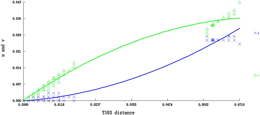
Substitution saturation test of nrDNA ITS sequences. The letters s and v represent transition and transversion, respectively.
3.2 Genetic diversity and divergence
All parameters linked to the genetic variation of ITS were estimated among the accessions. Genetic parameters were estimated by k, π, Hd, and θw, which exhibited values of 1.5944, 0.0027, 0.5405, and 0.0160, respectively (Table 4). The nucleotide datasets revealed moderate genetic diversity of nrITS among accessions. A total of 20 haplotypes were identified among 122 J. curcas individuals. The pairwise genetic divergence (GD) between ITS haplotypes was evaluated and ranged from 0.000 to 0.017, whereas the average of all haplotype sequences was 0.002. The GD value between H17 (MX2), H4 (CHGZ3), and H5 (CHGZ4) exhibited the highest divergence of 0.017.
Genetic diversity and neutrality test of all accessions based on the nrDNA ITS sequence data.
| Gene | n | k | π | Hd | θ w | Fu and Li's D | Fu and Li's F | Fu's Fs | Tajima's D |
| ITS | 123 | 1.5944 | 0.0027 | 0.5405 | 0.0160 | –8.25200 (P < 0.02) | –7.07538 (P < 0.02) | –4.768 (P < 0.005) | –2.62985 (P < 0.001) |
3.3 Neutrality tests and demographic history analysis
Neutrality tests were performed to determine whether the ITS region was subject to selection or evolved neutrally. Both values were investigated with Tajima's D and Fu and Li's tests. The value for Tajima's D was –2.62985 (P < 0.001), while that for Fu and Li’ s D was –8.25200 (P < 0.02) and that for Fu and Li's F was –7.07538 (P < 0.02; Table 4). The significant negative values suggest that the variation deviates from selective neutrality. To clarify the cause of deviation from neutrality, Fu's Fs was also estimated (Fu's Fs = –4.768; P < 0.005). Tajima's D, Fu and Li's, and Fu's tests consistently revealed significant negative values for J. curcas lineages, which supports selection and non-neutral evolution. This suggests a bottleneck effect and recent demographic expansion of intergenic spacers of ribosomal DNA in J. curcas accessions [26,27]. The mismatch distributions consisted of a significant unimodal curve (r = 0.0815; P = 0.5535) consistent with the hypothesis of sudden population expansion related to the distribution of J. curcas (Fig. 2).
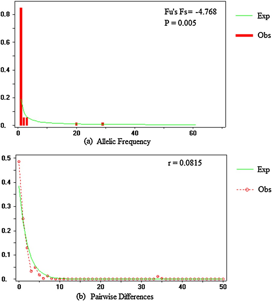
Mismatch distribution for nrDNA ITS sequences of J. curcas accessions. The number of pairwise differences and their frequencies are shown on the horizontal and vertical axes, respectively: a: spectrum frequencies of sites at nrDNA ITS sequences. The solid lines indicate the distributions under neutrality; b: mismatch distribution of the pairwise nucleotide differences for ITS sequences. The solid line represents the expected (Exp) mismatch distribution under a model of sudden demographic expansion and the mismatch observed (Obs) distribution with a dotted lines (r: ruggedness; p: probability).
3.4 Phylogenetic analysis
A 50% majority rule consensus tree was inferred from Bayesian analysis with posterior probabilities (PP). The parsimony analysis revealed 60 most parsimonious trees, with a consistency index (CI) of 0.9333 and a retention index (RI) of 0.9259. The MP topology (not shown) was congruent with the BI tree, which was well resolved (Fig. 3). The BI tree revealed a moderately resolved phylogeny and the J. curcas accessions were distinctly divided into three phylogeographic groups: Groups A, B, and C. Accessions of J. curcas in Group A were noticeably split into three major lineages: Clade I, Clade II, and Clade III, which were sister to Group B. Clade I included eight accessions: India (2), Madagascar (1), Cape Verde (2), and Mexico (3). Clade II consisted of 12 accessions: Brazil (1), Madagascar (1), Spain (1), Cape Verde (2), and Mexico (7). Clade III comprised 17 accessions: China (13), India (1), and Vietnam (3). Group B had a short branch and included 84 accessions: China (58), Burma (5), Indonesia (2), India (6), Laos (1), Thailand (4), Vietnam (4), Brazil (1), Burkina Faso (1), Mali (1), and Zambia (1). Group C consisted of an independent clade comprising a single Chinese accession (CHS1).

Bayesian-inference consensus tree of 122 accessions of J. curcas including one outgroup J. gossypifolia inferred from nrDNA ITS sequence data. Numbers before the backslash are posterior probability values and behind the backslash are bootstrap values. The hyphens denote that the clade is collapsed. Branch lengths are proportional to the number of nucleotide substitutions. The scale indicates the substitution rate.
The haplotype network revealed a significant genealogical relationship among J. curcas accessions, which was generally compatible with the phylogenetic analysis (Fig. 4). H11 was in the central position of the network and was composed of seven individuals from Spain (1), Cape Verde (2), and Mexico (4), connecting H2, H3, H13, H14, H16 and one missing haplotype. These additional haplotypes were one mutational step removed from H11 and exhibited a typical star-like genealogy structure, which suggests that H11 represent an ancestral haplotype [28]. Another single dominant haplotype (H1) was present in 82 individuals and distributed in a central position. This appeared to be a founder haplotype for H3, H6, H7, H8, and H13. This star-like pattern of H1 in the network suggests a rapid demographic expansion and evolution from a small founding population [28,29]. In addition, haplotypes H17, H18, H19, and H20 from Mexico were identified and exhibited numerous mutational steps from H11, suggesting remote phylogenetic relationship and significant genetic divergence among Mexican haplotypes.
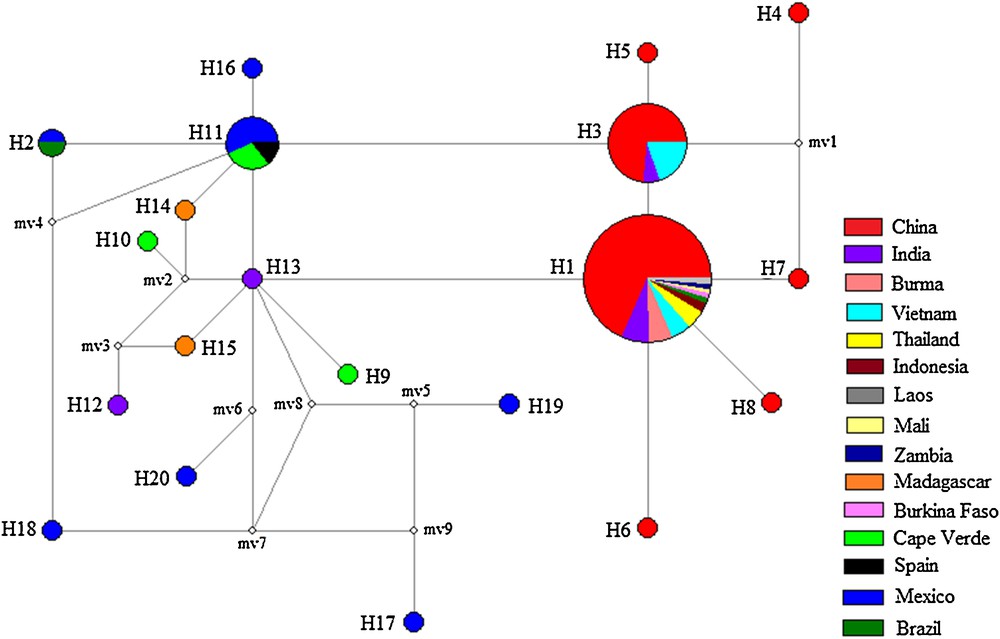
Median-joining network for J. curcas based on 20 nrDNA ITS Haplotypes. Sampled haplotypes are indicated by colored circles and designated by numbers. The inferred unsampled haplotypes are indicated by minimal white circles. Each line between two haplotypes represents a mutational step. Haplotypes are colored according to sites where the samples were collected. Circle size is proportional to the observed haplotype frequency.
4 Discussion
4.1 Genetic diversity and variation
Genetic diversity, estimated with k, Hd, π, and θw revealed a moderate amount of genetic variation and diversity. Variation in nrITS among J. curcas accessions revealed higher haplotype diversity (Hd = 0.5405) and lower nucleotide diversity (π = 0.0027), which may be associated with particular ecological conditions, a low level of recombination, and few base variations in the nuclear genome [30]. It is likely that the species encountered genetic bottlenecks and founder effects during its geographic spread [31,32]. The highest level of genetic divergence was evaluated as 0.017 between haplotypes H17 (MX2), H4 (CHGZ3), and H5 (CHGZ4), and the genetic distances between Mexican haplotypes were evidently higher than those of other regions (Table 5). There was significant genetic divergence between Mexican and Asian, African, and South American haplotypes, suggesting restricted gene flow between adjacent populations caused by geographical isolation, abundant vegetative propagation, and asexual reproduction [11–13].
Estimates of pairwise genetic divergence (GD) between the 20 Haplotypes of J. curcas based on nrDNA ITS sequence data.
| H1 | H2 | H3 | H4 | H5 | H6 | H7 | H8 | H9 | H10 | H11 | H12 | H13 | H14 | H15 | H16 | H17 | H18 | H19 | H20 | |
| H1 | ||||||||||||||||||||
| H2 | 0.003 | |||||||||||||||||||
| H3 | 0.002 | 0.002 | ||||||||||||||||||
| H4 | 0.005 | 0.005 | 0.003 | |||||||||||||||||
| H5 | 0.005 | 0.005 | 0.003 | 0.007 | ||||||||||||||||
| H6 | 0.000 | 0.003 | 0.002 | 0.005 | 0.005 | |||||||||||||||
| H7 | 0.002 | 0.005 | 0.003 | 0.003 | 0.007 | 0.002 | ||||||||||||||
| H8 | 0.000 | 0.003 | 0.002 | 0.005 | 0.005 | 0.000 | 0.002 | |||||||||||||
| H9 | 0.007 | 0.007 | 0.008 | 0.012 | 0.012 | 0.007 | 0.008 | 0.007 | ||||||||||||
| H10 | 0.002 | 0.002 | 0.003 | 0.007 | 0.007 | 0.002 | 0.003 | 0.002 | 0.005 | |||||||||||
| H11 | 0.003 | 0.000 | 0.002 | 0.005 | 0.005 | 0.003 | 0.005 | 0.003 | 0.007 | 0.002 | ||||||||||
| H12 | 0.002 | 0.002 | 0.003 | 0.007 | 0.007 | 0.002 | 0.003 | 0.002 | 0.005 | 0.000 | 0.002 | |||||||||
| H13 | 0.002 | 0.002 | 0.003 | 0.007 | 0.007 | 0.002 | 0.003 | 0.002 | 0.005 | 0.000 | 0.002 | 0.000 | ||||||||
| H14 | 0.003 | 0.000 | 0.002 | 0.005 | 0.005 | 0.003 | 0.005 | 0.003 | 0.007 | 0.002 | 0.000 | 0.002 | 0.002 | |||||||
| H15 | 0.002 | 0.002 | 0.003 | 0.007 | 0.007 | 0.002 | 0.003 | 0.002 | 0.005 | 0.000 | 0.002 | 0.000 | 0.000 | 0.002 | ||||||
| H16 | 0.007 | 0.003 | 0.005 | 0.008 | 0.008 | 0.007 | 0.008 | 0.007 | 0.010 | 0.005 | 0.003 | 0.005 | 0.005 | 0.003 | 0.005 | |||||
| H17 | 0.012 | 0.012 | 0.013 | 0.017 | 0.017 | 0.012 | 0.013 | 0.012 | 0.015 | 0.010 | 0.012 | 0.010 | 0.010 | 0.012 | 0.010 | 0.015 | ||||
| H18 | 0.007 | 0.003 | 0.005 | 0.008 | 0.008 | 0.007 | 0.008 | 0.007 | 0.010 | 0.005 | 0.003 | 0.005 | 0.005 | 0.003 | 0.005 | 0.007 | 0.008 | |||
| H19 | 0.008 | 0.008 | 0.010 | 0.013 | 0.013 | 0.008 | 0.010 | 0.008 | 0.012 | 0.007 | 0.008 | 0.007 | 0.007 | 0.008 | 0.007 | 0.012 | 0.010 | 0.008 | ||
| H20 | 0.007 | 0.007 | 0.008 | 0.012 | 0.012 | 0.007 | 0.008 | 0.007 | 0.010 | 0.005 | 0.007 | 0.005 | 0.005 | 0.007 | 0.005 | 0.010 | 0.012 | 0.007 | 0.012 |
4.2 Phylogenetic relationships and intraspecific divergence
The combined results of the phylogenetic and network analyses were moderately resolved, and the accessions of J. curcas were consistently divided into three genetically distinct population lineages (Groups A, B, and C). Group A was separated into Clades I, II, and III and included all the primary Mexican accessions. Group B was composed of the major lineage accessions from Asia, especially from southern and southwestern China. Combined with the data from the network analysis, our results suggest that the American and Asian accessions of J. curcas were identified as two distinct nuclear ribosomal lineages. Phylogenetic relationships between American and Asian lineages demonstrated remote geographical isolation and restricted gene flow, generating significant genetic divergence between American accessions and accessions from other regions [11,13,33].
BI phylogenetic trees showed that the primary American lineages (Mexico and Brazil) were clustered together with accessions from Cape Verde, Spain, Madagascar, and India, forming a distinct sister subgroup with the Asian lineage (China, India, and Vietnam). This suggests a relatively close phylogenetic relationship and evolutionary history and indicates that the Asian lineage may have originated from the American lineage [11,13,14]. The phylogenetic trees showed that accessions from Asia, Africa, and South America clustered together with extremely short internal branches in Group B, and shared a single dominant haplotype (H1). This indicates high genetic similarity a common origin, and a slow rate of genetic divergence among population lineages, suggesting a rapid radiation and recent demographic expansion caused by a founder effect [31,32]. The pattern of haplotype diversity, the significant negative values for the neutrality tests, and the mismatch distribution were consistent with this conclusion. Both the phylogenetic trees and the network analysis identified the presence of two separate lineages among the Chinese accessions, indicating that China's complicated geography and diverse ecosystems led to restricted dispersal and gene flow, and promoted genetic diversification in southwestern China [34].
4.3 Geographic origin and dispersal route
J. curcas is believed to be native to Central America or Mexico, where it occurs naturally in forests in coastal regions [35]. It was then perhaps widely disseminated from its center of origin by the Portuguese, who transported it to the Old World [3]. The Ceara State in Brazil was also identified as a possible center of origin; however, this proposal was unfounded [36]. Despite this, the center of origin of J. curcas has remained controversial for many years. Our data confirms that Mexico or Central America is the center of biodiversity and the possible center of origin, due to the dominant haplotype frequency and the high genetic variability of accessions from this area [7,13].
Regarding the migration route, texts have mentioned the use of J. curcas prior to 1810 [3]. Previous research assumed that the Portuguese distributed J. curcas from the Caribbean via Cape Verde to Africa and Asia [3,14]. However, the migration and dispersal route remained uncertain. Our BI tree showed initial clustering of CV3 and MX1 (in Clade II of Group A), followed by the formation of a sister subclade, which suggests that the Cape Verdean accessions had prior phylogenetic relatedness with Mexican accessions, and then with the Spanish accessions. The cluster of CV2 (or CV1) and MA2 in Clade I indicates the close relationship between Cape Verdean and Madagascan accessions. Meanwhile, the genetic divergences between H1 and H14 and between H1 and H15 were 0.003 and 0.002, respectively, suggesting that accessions from Madagascar are closely related to Asian accessions, especially to the Chinese accessions. Furthermore, one Brazilian and three African accessions clustered with Asian accessions in Group B and shared one common haplotype in H1, suggesting their close relatedness and migratory connectivity. Combining the above data analyses, we deduced that J. curcas was distributed from Mexico through the Caribbean and/or Brazil by the Portuguese, via Cape Verde where there was a presumed bifurcation point, with one route going to Spain and then to China, further spreading to other regions of Southeast Asia. Another route was dispersed to Africa, via Madagascar and migrated to China, and then further spread to other regions. Our research tentatively supports previous research and provides further details of the migration route (Fig. 5).
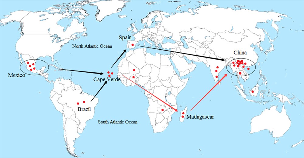
The putative migratory route of J. curcas deduced by nrDNA ITS sequence data analysis.
5 Conclusion
Phylogenetic relationships and intraspecific divergences of J. curcas were elucidated, and our results suggest distant geographical isolation and genetic divergence between American accessions and other accessions. Furthermore, we also demonstrated that Mexico or Central America is the possible center of origin, and we deduced the putative migration route. These results expand the current understanding of J. curcas and may aid in genetic improvement and the development of breeding programs.
Disclosure of interest
The authors declare that they have no competing interest.
Acknowledgments
The research was supported by grants from the National “12th Five-Year” Science and Technology Support project of China (No. 2011BAD22B08). The authors would like to thank the editors and the anonymous reviewers for helpful comments and suggestions to improve the manuscript.