

1 Introduction
Polymer latices have long been important items of commerce and are produced in very large quantities throughout the world. Most of these are aqueous based and find application as impact modifiers, coatings, adhesives and in medical diagnostics. Their property advantages derive from their particulate nature (particles commonly in the range of 50–500 nm) and high molecular weights. In addition, many of these polymer systems are composites of two or more incompatible polymers displaying specific morphological structures within the latex particles. For such systems the physical structure within the particles needs to be controlled at the scale of 20–100 nm, and there is always a fairly high percentage of the two polymers within the interfacial regions between the two polymers. Our interest has been in latex particle morphology control and the phase separation processes that produce such structures. We typically produce polymer latices via the free radical polymerization mechanism and employ reaction temperatures in the 60–90°C range. In such systems, we begin with a simple polymer latex (usually a copolymer) with controlled particle size – called seed latex – and then polymerize a second polymer within those seed latex particles. In most cases, the newly formed polymer phase separates from the seed polymer throughout the reaction. How this phase separation process occurs is the subject of this paper.
Phase separation within polymer solutions is usually treated by applying the concepts of solution thermodynamics to a three-component system composed of two polymers and a solvent (in our case the solvent is the monomer of the second polymer). The simple phase diagram for such a system (the two polymers are considered to be completely immiscible without a co-solvent) is shown in Fig. 1 where we display the binodal and spinodal curves. A reaction process pathway is also shown in the figure to demonstrate the overall composition within the system during the reaction (in this case it is for a batch reaction starting with equal amounts of seed polymer and second stage monomer). As the reaction drives the overall composition into the two-phase region, phase separation occurs. Using solution thermodynamics this situation is usually described on the free energy versus composition plot as the common tangent points (specifying the binodal points) and the inflections points in the curve specifying the spinodal points. When phase separation happens at compositions within the space between the binodal and spinodal points, the mechanism is judged to be nucleation and growth (NG). If phase separation happens deeper within the two-phase region, the mechanism is spinodal decomposition (SD). Nucleation and growth requires the process to overcome an energy barrier, while spinodal decomposition is a spontaneous process with no energy barrier.
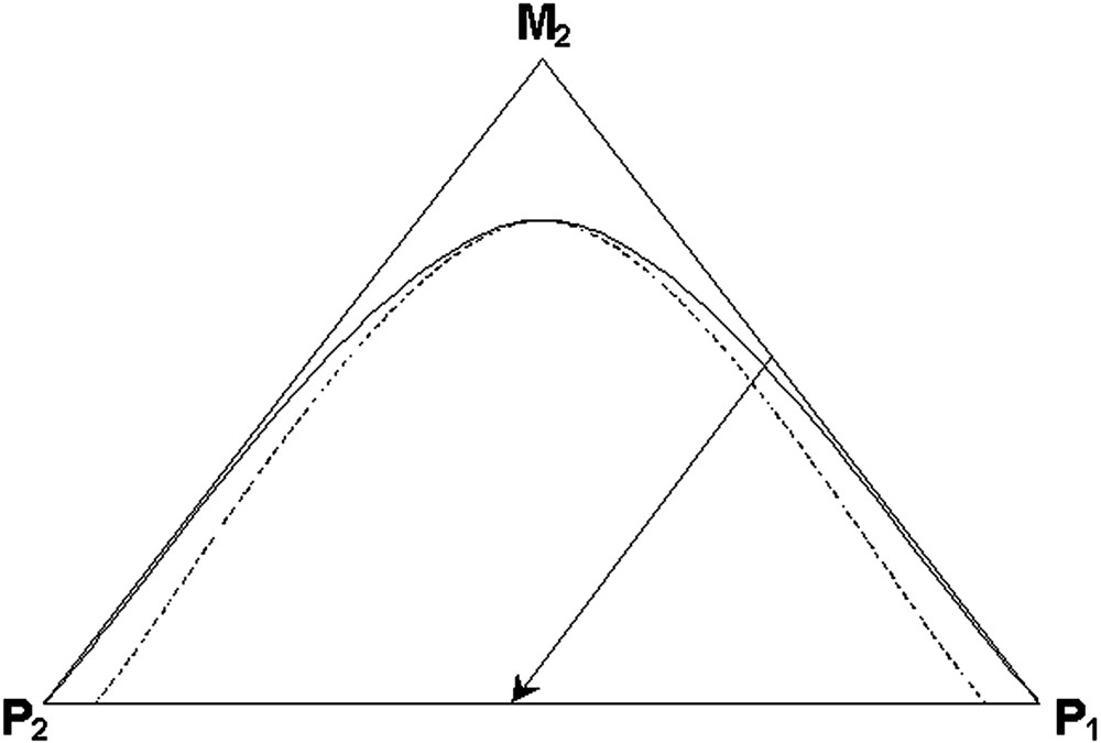
Three-component phase diagram with a batch reaction pathway.
Phase separation driven by a polymerization reaction (generically called polymerization induced phase separation, or PIPS [1]) has been discussed in the literature utilizing both the SD and NG mechanisms to describe the process. Chan and coworkers [2,3] have treated a condensation polymerization system undergoing phase separation via SD and have provided greatly detailed models of the individual polymer concentration profiles within the material as they change with reaction time. Such predictions are computationally intensive and result in morphology characterized by uniformly shaped and sized domains (or occlusions) randomly distributed in a bulk (macroscopic) matrix. Alternatively, Williams et al. [4] have treated a bulk condensation polymerization system containing dissolved rubber and used the NG mechanism to describe the manner in which the rubber phase separated from the reacting fluid. They computed the critical size of the nucleated droplets of rubber phase and how the droplet sizes changed with the reaction time. In contrast to the work by Chan [2,3] where the second stage polymer separated from the reacting solution, in Williams’ system the first, or seed, polymer phase separated from the other. This was due to the starting compositions of seed polymer and second stage monomer. An and Sperling [5] treated the development of multiphase morphology during polymerization of sequential IPNs and suggested that in the bulk system the early phase separation likely takes place via NG, followed shortly by a switch to a ‘modified’ SD mechanism. They did not model the polymerization reaction dynamics and only treated a generic, bulk system. Lastly, Sigalov and Rozenberg [6] treated another polycondensation system containing a second non-reacting polymer and provided a modeling framework using the NG mechanism. However they did discriminate between the application of the SD and the NG mechanisms by commenting that the former applied to reacting systems in which the rate of reaction is much faster than the rate of phase separation (or polymer diffusion), while NG applies to systems in which the opposite is true.
In all of the literature we have surveyed, there is no discussion of phase separation via NG or SD in latex particles undergoing either batch or semi-batch reactions of the second-stage monomer. Nor have we seen any modeling of phase separation within systems in which the reactions occur by the free radical mechanism. Our work involves free radical polymerization and the resultant phase separation within latex particles with diameters in the 100–350 nm range. These process conditions are depicted as the reaction paths in Fig. 2 . Here it should be noted that at high monomer feed rates (and for batch reactions), phase separation takes place initially in a relatively low viscosity medium. When the monomer feed is stopped, the viscosity continuously increases during the remainder of the reaction and phase separation must occur under variable conditions. Also, because the monomer is easily distributed between the two phases within the particle, polymer radicals may exist in both phases and thus reaction occurs in both phases throughout the polymerization process. At very slow monomer feed rates (the so-called ‘starve-fed’ condition), the instantaneous monomer concentration is very low throughout the entire reaction and thus phase separation must occur in a very viscous medium. On the one hand, such process systems allow us to study phase separation over a wide variety of conditions for the same polymer system, and on the other hand we are presented with a formidable challenge.
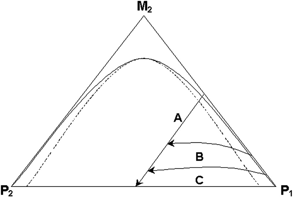
Three-component phase diagram with batch and various semibatch reaction pathways.
We have done many investigations of latex particle morphology under conditions in which the polymer reactions are slow enough that phase separation achieves its thermodynamic equilibrium state [7–15]. In this state the final particle structure is determined by the minimization of the interfacial free energies of the various polymer interfaces within and at the extremity of the particle. More recently we have studied a number of systems in which the morphology is developed under non-equilibrium conditions characteristic of high viscosities during the reaction [16–21]. In these cases polymer diffusion rates and reaction rates together determine the morphology. It is with this latter set of studies that we have come to question where (within the particle) and how (NG or SD) phase separation takes place. As a first step we have applied the NG concepts to several latex systems to determine whether or not such an analysis offers results that reasonably agree with the non-equilibrium structures that we obtain for such systems. This analysis and comparison is the purpose of this paper.
2 Theoretical considerations
Here we evaluate the nucleation and growth possibility by applying theoretical predictions to real experimental systems and comparing these to the domain sizes as observed in transmission electron microscopy (TEM). The thermodynamic relations governing the size of nucleated domains are well known, and the methodology for applying this to polymer systems has been presented [4]. For a two component system containing two polymers, 1 and 2, the partial molar free energies, , of each component are given by [22,23]:
| (1) |
| (2) |
| (3) |
In a latex particle during a second stage polymerization, we are dealing with a three-component system consisting of polymer 1, polymer 2 and monomer 2. For the three-component system, the partial molar free energies of all three components can be written and the free energy of mixing determined. The solution of this system of equations typically requires numerical methods [22]. However, by making a few simplifying assumptions, useful approximations are obtained that allow one to gain an understanding of certain types of simple three-component systems. One such simplification has been referred to as the ‘special symmetrical case’ [22], and in this case it is assumed that μ10=μ20, and that N1 =N2 =N (the subscript 0 refers to the monomer, or solvent. The assumption of equal interaction parameters between each polymer and the monomer means that the monomer will distribute equally between both polymer phases, which is a reasonable assumption in many systems. By making these assumptions, the system can be described as a pseudo-two-component system. In this case the volume fractions of each polymer are defined as:
| (4) |
| (5) |
| (6) |
| (7) |
The above equations allow us to describe the free energy for a given polymer – polymer – monomer system and identify the binodal (the points having a common tangent, which are the minimum points for the symmetrical case) and spinodal (inflection points) concentrations. Phase separation occurring between the binodal and spinodal concentrations will occur by the nucleation and growth mechanism. The method for predicting the nucleus size in polymer systems was outlined by Williams [4]. For this purpose, it is useful to write the free energy on a volume basis, rather than the molar basis used in Eq. (3). This is done by introducing the molar density, , such that:
| (8) |
| (9) |
The mixing free energy per volume gained by phase separating polymer 2 from a mixture of polymers 1 and 2 is defined as ΔGN and is given by:
| (10) |
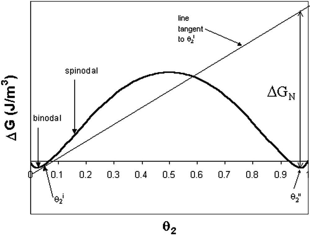
Gibbs energy of solution for the special symmetrical case of two polymers and one solvent (monomer). The method to determine ΔGN is illustrated.
Once ΔGN is known, the size of a nucleated domain can be determined. Since phase separation requires the formation of a new interface, and this interface has an energy associated with it (interfacial tension), the size of the nucleus is determined by balancing these energies. This leads to:
| (11) |
| (12) |
In order to predict nucleus sizes, several parameters are required, namely μ12, γ, N and φ0. To evaluate the model and its sensitivity to these parameters, we applied the treatment to a simple system of poly(methyl methacrylate)/polystyrene (PMMA/PS). Estimates of γ were obtained by methods outlined by Wu [24]. The value of μ12 is determined from solubility parameters as follows [25]:
| (13) |
Calculated nucleus sizes for a representative PS/PMMA system
| Parameter | Parameter value | DN, diameter of nucleus (nm) |
| Fraction of spinodal | 0.01 | 15.8 |
| " | 0.1 | 15.4 |
| " | 0.5 | 15.2 |
| " | 0.99 | 15.1 |
| Molecular weight, M | 100 000 | 20.5 |
| " | 500 000 | 15.4 |
| " | 1 000 000 | 14.8 |
| φ0, monomer volume fraction | 0.05 | 15.4 |
| " | 0.5 | 47.9 |
| Interfacial tension, γ (mN m–1) | 1.0 | 7.7 |
| " | 2.0 | 15.4 |
| " | 4.0 | 30.8 |
| Solubility parameter for PS | 18.3 | 8.4 |
| δps | 18.5 | 12.9 |
| 18.57 | 15.4 | |
| 18.9 | 48.9 | |
| 19.0 | 86.7 | |
| 19.2 | 2244 |
The values in Table 1 show that the size of the nucleus does not depend greatly on the choice for the volume fraction of the initial solution before phase separation, θ2i(described in Table 1 as the fraction of the spinodal concentration). For the remaining discussion in this article, the value of θ2iwas taken to be 10% of the spinodal concentration for convenience when comparing different systems. Table 1 also shows that the nucleus size does not vary greatly with the molecular weight within the range shown, which are typical molecular weights for polymers produced by emulsion polymerization. The variation is much greater for the monomer volume fraction, although this change is overestimated because in reality an increase in the monomer concentration will result in a subsequent decrease in the interfacial tension, which will result in smaller domain sizes. As expected, fairly significant changes are noted with variation in the interfacial tension, with larger values resulting in larger nucleus sizes.
The first four parameters in Table 1 are relatively straightforward to determine or estimate in order to make predictions for real systems. However, as indicated by the standard deviation on the solubility parameters, these values, and hence the interaction parameter, are not known with a high level of confidence. This is particularly problematic because the value of the nucleus size varies greatly with changes in this parameter. It should be noted that the change in the solubility parameter for polystyrene in Table 1, from 18.57 to 19.2, is well within the standard deviation of the values obtained from the literature. This results in a change of two orders of magnitude for the predicted nucleus size. Therefore, careful attention must be paid to the estimation of the interaction parameter in order to obtain reasonable predictions for nucleus sizes in real systems.
At this point, it is also necessary to consider what happens to the nucleated domains during the remainder of the polymerization process. We know that nucleated domains formed early in the reaction can continue to grow by polymerization, and thus we expect a distribution of domain sizes at the end of the process. With this in mind, we have established a mathematical relation to calculate the size range of these phase-separated domains at the end of the polymerization.
We consider a latex particle of initial diameter D0 composed of seed polymer P1. A second stage monomer M2 is fed to the reactor and polymerizes within the P1 particles, forming polymer P2. We consider the typical semi-batch case where monomer M2 is fed slowly so as to control the rate of polymerization. Due to this resulting balance between polymerization rate and monomer feeding rate, a steady state concentration of monomer is reached inside the particle (outside of the very early and late stages of this semi-batch polymerization). Therefore, the size of the nucleated domains will be fairly constant throughout the polymerization process.
Furthermore, we consider that a region of space may exist within the core of the particles, where radicals cannot be present under polymerization conditions. This is because a typical emulsion polymerization uses a water-soluble initiator, so oligomeric radicals enter from the water phase, and under many conditions diffusional restrictions prevent them from fully penetrating into the interior of the particles. This region where no radicals exist is related to the fractional penetration ratio, FP. FP is defined as the distance into the particles that radicals can diffuse, divided by the radius of the particle. Hence, a fractional penetration significantly less than one indicates that radicals cannot penetrate the particle (i.e. only a shell can be developed), while a value of FP greater than or equal to one indicates a system in which radicals can fully penetrate the particle. This fractional penetration concept has been described in detail previously [17,20]. Under cases where radical penetration is limited, polymer nuclei can develop only in the ‘outer region’ of the particle.
Early in the polymerization, after some level of conversion X1, a sufficient amount of second-stage monomer has been polymerized to create the first nucleus of diameter DN, as calculated from Eq. (12). The quantity of polymer in this nucleus and the overall conversion at this point in time is determined by Eq. (14).
| (14) |
Let us now consider the case of a particle already containing i nuclei, all of them having undertaken growth, at the level of conversion Xi. The incremental amount of conversion to create a new nucleus ‘i + 1’ is Xi+1−Xi. This amount corresponds to the same amount of material necessary to create the initial nucleus ‘1’ of diameter DN, plus the amount of polymer that has polymerized inside the other pre-existing nuclei during this conversion increment. This results in Eq. (15).
| (15) |
| (16) |
When combining Eqs (14)–(16), we obtain Eq. (17):
| (17) |
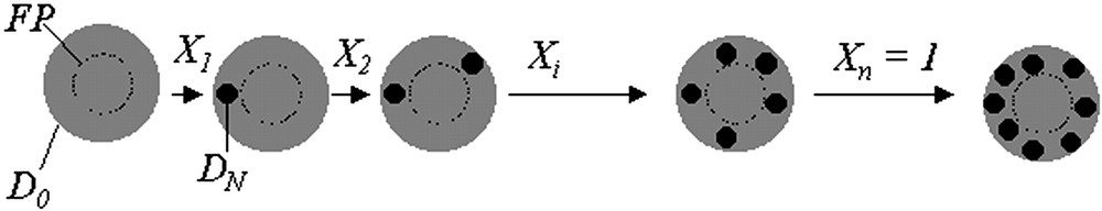
Schematic illustration of a nucleation and growth mechanism occurring in the outer region of a latex particle.
Further equations can be derived from Eq. (17) and solved to determine the number of domains that will be formed within each latex particle throughout the polymerization, but this is not included here for the sake of brevity. Furthermore, an expression can easily be developed to calculate the maximum size of a domain produced by nucleation and subsequent growth by polymerization. The largest possible domain (excluding domain reconsolidation by Oswald ripening) is the first domain to have been nucleated (at conversion X =X1), which has undergone continuous growth (from X =X1 to X = 1). The smallest domain observable remains the last domain to have been nucleated, of diameter Dc. The diameter, Dmax, of the largest domain can be calculated as:
| (18) |
3 Experimental details
In this study we chose to work with a system in which the phase-separated domains could be easily distinguished. Thus we selected acrylic/styrene-based composites for which we could easily stain the styrene-containing polymer with ruthenium tetraoxide prior to observation of the microtomed sections of the particles in a transmission electron microscope (TEM). We also chose to work at relatively large particle sizes so that they could be easily seen in the TEM Photos. In addition, we used acrylic seed latices whose copolymer would be glassy during the reaction conditions. In this way, we conjectured that there would be little chance for phase rearrangement, or ripening, during or after polymerization, thus preserving the phase structure for TEM observation.
Here we describe four different latex systems in which the seed copolymers, composed of methyl acrylate (MA) and methyl methacrylate (MMA) vary in their dry state Tg. This was achieved by varying the co-monomer ratios. We used batch, surfactant-free emulsion polymerization techniques to create all seed latices. Small amounts of SDS surfactant were added midway through the reactions to provide for colloidal stability. Since the seed latices were prepared by batch reactions, and due to the differences in the copolymerization reactivity rations of the MA and MMA monomers, it is likely that some level of compositional drift has occurred during the polymerizations. DSC analysis of each seed copolymer showed only slightly wider transitions than expected for perfectly statistical copolymers (run under the same DSC conditions, with a heating rate of 10 °C min–1), and in each case only a single glass transition was detected. Thus we do not expect major compositional gradients within the seed particles. Prior to second-stage polymerizations, the seed latices were cleaned by mixing the latex with ion exchange resins (mixed bed) and characterized for copolymer ratio (via NMR) and particle size distribution (via CHDF).The second stage reactions were conducted at 70 °C and styrene monomer was fed to a 250-ml glass reactor over different lengths of time. Potassium persulfate was used as the initiator and was added once at the beginning of the second stage reaction. Table 2 provides the recipes used for the seed latices and Table 3 provides similar information for the second-stage lattices [27].
Seed latex recipes
| Seed number | MMA/MA | MMA | MA | Water | KPSa | NaHCO3a |
| ratio (wt/wt) | (g) | (g) | (g) | (mol l–1) × 103 | (mol l–1) × 103 | |
| LEI-18 | 80/20 | 56.1 | 14.1 | 930 | 3.2 | 6.5 |
| LEI-10 | 70/30 | 49.0 | 21.1 | 930 | 3.2 | 6.4 |
| LEI-4 | 60/40 | 60.0 | 40.1 | 930 | 3.2 | 6.7 |
| LEI-36 | 40/60 | 28.8 | 42.0 | 930 | 3.2 | 6.4 |
Second-stage reaction recipes
| Experiment | Seed latex | Seed polymer Tg (°C) | Seed particle diameter (nm) | Stage ratio (SR) (styrene monomer: seed polymer) (wt/wt) | Styrene feed time (h) |
| A | LEI-4 | 77 | 390 | 1:1 | 9.6 |
| B | LEI-36 | 52 | 380 | 1:1 | 4.2 |
| C | LEI-18 | 98 | 330 | 1:1 | 4.2 |
| D | LEI-10 | 88 | 320 | 1:1 | Batch |
The morphological structures of the final latex particles were determined by air drying the latex to obtain a powder, and then embedding the powder in Epon 812 epoxy, which was cured overnight at 60 °C. These samples were microtomed to obtain sections of about 90-nm thickness, stained with ruthenium tetra-oxide vapor for about 10 min at room temperature, and observed in the TEM (Hitachi H-600) at about 80 keV. Further experimental details are provided elsewhere [18,19].
4 Discussion
The TEM photos of microtomed sections of the latex particles from the latices of experiments A through D are shown in Figs 5–8 respectively. It is clear that in each of these experiments, the particle morphologies are very different. The reasons for the formation of different morphologies is not the concern of this paper, and is discussed in detail elsewhere [18,19]. There is one common feature of each experiment however, which is that each morphology represents some sort of occluded structure, in which many separate domains of the second stage polystyrene are dispersed within the seed polymer phase. This is most obvious for the particles in Figs 5, 6 and 8. At first glance, Fig. 7 appears to display a classical ‘core-shell’ morphology. In general this is true, however, deeper inspection of the particles in Fig. 7 reveals a variation to the classic core shell structure in that the shell itself is composed of many small domains of polystyrene rather than being a continuous shell. Fig. 5 shows a morphology similar to that in Fig. 7, except that the domains within the shell are much more clearly distinguished.
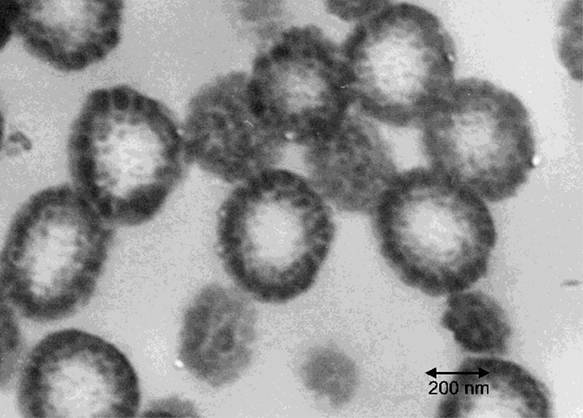
Microtomed TEM photo for Experiment A. The dark phase is the second-stage polystyrene.
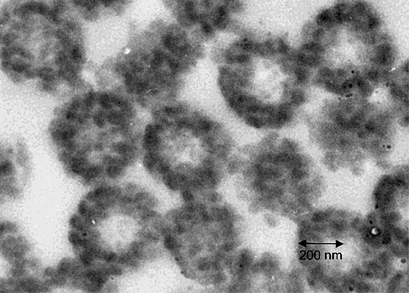
Microtomed TEM photo for Experiment B. The dark phase is the second-stage polystyrene.
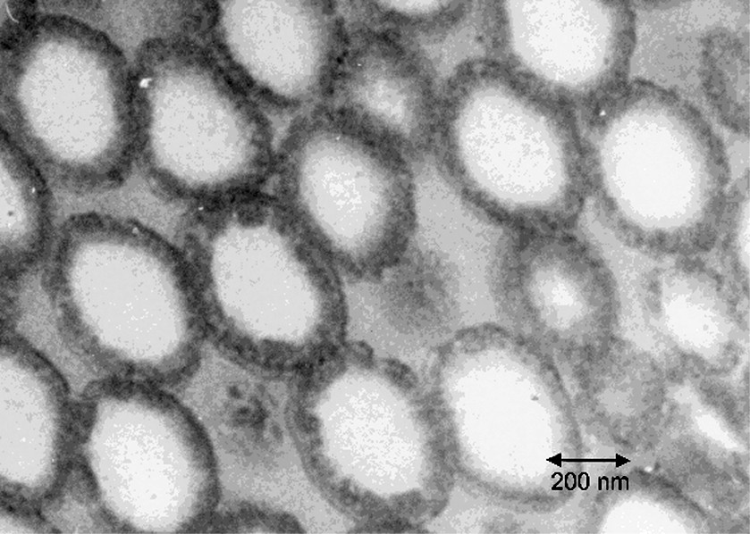
Microtomed TEM photo for Experiment C. The dark phase is the second-stage polystyrene.
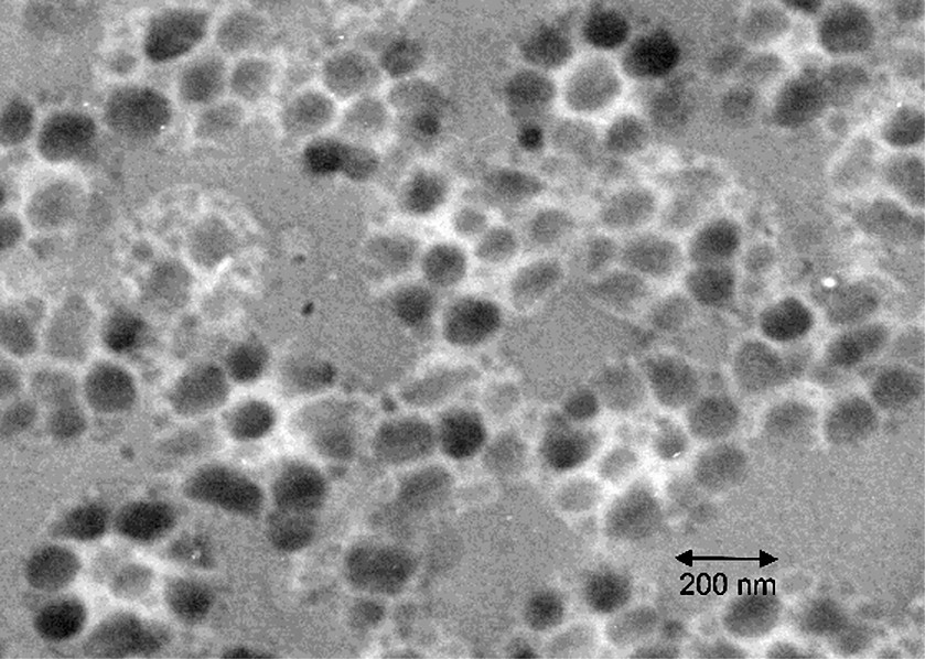
Microtomed TEM photo for Experiment D. The dark phase is the second-stage polystyrene.
The fact that all of these morphologies are some variation of an occluded structure is what makes these experiments particularly interesting in the context of this paper. They present a clear opportunity to compare predictions for the expected domain sizes based on the nucleation and growth models to real systems. One difficulty in applying the models, as described above, is in determining the interaction parameter, μ12, because of the inherent uncertainty in this parameter and the large impact that it has on the predicted nucleus sizes. The following approach was taken to overcome this difficulty. The domain sizes in Fig. 5 for Experiment A are particularly clear and, to the best of our ability, we have measured them to range from 30 to 50 nm. This experiment was used in order to fit the value of μ12 (or δPS) so that the maximum domain size after growth of the nuclei during polymerization, as calculated from Eqs (6) through (10) and (12), corresponds to the largest domains observed in the TEM (50 nm). The fitted value of δPS required was found to be 18.75 MPa1/2. This agrees well with the average value obtained from the literature (18.57) and is well within the standard deviation of the literature values (±2.6). This fitted value of δPS, and thus μ12, was then used for all of the subsequent calculations for the other experiments. It is noted that fitting the largest domain observed in the TEM to the largest domain expected by growth is perhaps not the most desirable approach to fit δPS. Since δPS is directly involved in predicting the nucleus size, it would be more desirable to fit the minimum domain size observed (which would correspond to a nucleated domain that has not experienced growth) to the value of the predicted nucleus size. However, for practical reasons involving the identification of domains in the TEM images, we have judged that it is more reliable to measure the largest domains observed and thus have used this approach in order to fit δPS.
As discussed above, in order to calculate the expected growth of the nucleated domains due to polymerization it is necessary to determine a fractional penetration value, which recognizes that in many cases the polymerization was confined to only the outer regions of the particles. For this purpose, we used the techniques described by Stubbs et al. [28] and Karlsson et al. [29] to simulate the reaction kinetics and radical penetration behavior during polymerization in each experiment of Table 3. These simulations also provide information about the concentration of monomer in the particles during the experiments, which is necessary to predict the nucleus sizes. Experiments A, B and C were all run under semibatch conditions so that the monomer concentrations were essentially at steady state during the entire polymerization. For this reason, one calculation for the expected nucleus size can be used to describe the conditions prevalent throughout the polymerization. This is not the case for Experiment D however. Since this polymerization was performed in a batch manner, the monomer concentration was very high at the beginning and decreased continuously throughout the polymerization. Therefore, for this experiment, calculations were made for two different conditions of monomer concentration, one high and one low, to predict the nucleus sizes expected at the early and late stages of the reaction, respectively.
All calculations considered the degree of polymerization, N, to be 5000. The molecular weights were not measured for these experiments, but this value is reasonable for polymers produced by emulsion polymerization without the use of chain transfer agents. This simplification is not considered to be critical, as the results in Table 1 show relatively little variation of the nucleus size with variations of the polymer molecular weight over this range. The interfacial tension, γ, used in most cases was 2.5 mN m–1, which was estimated using the harmonic mean equation as outlined by Wu [24]. In the case of the batch experiment at low conversion, the monomer concentration is very high and this will tend to decrease the interfacial tension between the two phases. For this condition, the value of γ was estimated from the correlations presented by Winzor et al.[10] to be 1.4 mN m–1. The values used to make predictions for each experiment, as well as the predicted nucleus sizes and maximum domain sizes due to growth are given in Table 4. Also included are the measured domain sizes for the actual experiments, as determined from the TEM photos in Figs 5–8. It is noted that the estimation of the domain sizes is subject to a certain level of uncertainty as it is not always completely clear where to define the ‘edge’ of a domain, due to the presence of finite interfacial widths between the two polymer phases. Another difficulty is the fact that the volume fraction of P2 domains in the outer region of the particles is quite high in several cases, and this leads to overlap of domains in the cross section and creates difficulty clearly distinguishing one domain from another. Identification of individual domains was particularly difficult in the case of Experiment C (Fig. 7), where the separate domains in the shell of the particle are much more difficult to distinguish clearly. Therefore, we view the measured domain sizes for this particular experiment with significantly more uncertainty than the others.
Calculated nucleus and maximum domain sizes, and comparison to experimental data
| Experiment | A | B | C | D | D |
| → | Low conv. | High conv. | |||
| [M] (mol l–1) | 0.16 | 0.45 | 0.6 | 5.0 | 1.0 |
| φ0 | 0.017 | 0.048 | 0.064 | 0.53 | 0.107 |
| γ12 (mN m–1) | 2.5 | 2.5 | 2.5 | 1.4 | 2.5 |
| FP | 0.11 | 0.41 | 0.13 | 1.0 | N/A |
| DN (nm) | 31 | 33 | 34 | 68 | 37 |
| Dmax (nm) | 50 | 43 | 53 | 86 | N/A |
| Measured max. domain size (nm) | 50 | 50 | 50 | N/A | 110 |
| Measured min. domain size (nm) | 30 | 30 | 30 | N/A | 30 |
For Experiment A, the values for both the predicted and experimental maximum domains sizes are in bold type. This is because this condition was used to adjust the interaction parameter for the system, and is the reason that the two values are identical. However, it is interesting to note that the nucleated domain size predicted for Experiment A of 30nm corresponds to the smallest domain that was measured by TEM. This result, that the range of domain sizes observed in the TEM corresponds to the range predicted by nucleation and growth, is not predetermined by the fitting procedure. The results are very similar for Experiments B and C in that the minimum and maximum domain sizes measured in the TEM correspond well to the predicted nucleus sizes and maximum domain sizes due to growth by polymerization.
For Experiment D, several features are clear in the TEM image of Fig. 8. The first is that the PS domains are distributed throughout the entire particle volume, as opposed to experiments A-C in which they are preferentially located in the outer regions of the particle. This is because Experiment D was run in a batch manner, so the monomer concentration was much higher during the majority of the polymerization. This gives rise to much higher diffusion rates for the entering radicals, and hence they are able to fully penetrate into the center of the particles. The remaining features observed in Fig. 8 are related to the sizes of the PS domains. It is clear that (1) much larger domains are observed than in the other experiments and (2) a much larger variation in domain sizes is evident, as both large and small domains are observed. This is reflected in the domain size measurements displayed in Table 4. The predicted domain sizes for both the low and high conversion cases for the batch experiment may help to explain these features. First, it is seen that the domain sizes expected at low conversion are much larger than at high conversion. At low conversion, the nucleated domains are expected to be about 68 nm, and if they continue to grow by polymerization they may reach a size of about 86 nm. However, nucleated domains formed at high conversion will be in the range of 35–40 nm, and these will not have a chance to grow by further polymerization. Therefore, the expected range of domain sizes would be between 35 and 85 nm. The measured domain sizes reveal that there is in fact a large range as expected, but that the maximum domain sizes observed are much larger than what would be expected due to growth by polymerization. This suggests that significant consolidation of phase separated domains has occurred during the polymerization, either by the mechanism of Ostwald ripening or by coalescence of separate domains. The fact that the monomer concentration is higher in the batch experiment than the semibatch experiments means that diffusion of the polymer chains occurs more easily, and this seems to have allowed for consolidation of phase separated domains. We now feel that this is one useful application of this simple nucleation and growth model for phase separation. When the observed domain sizes are significantly larger than what would be expected due to nucleation and growth by polymerization alone, it can be deduced that significant ripening of the phase separated morphology has likely occurred.
The results of Table 4 show that the nucleation and growth treatment yields very reasonable predictions for the size of the nucleated domains as well as their expected level of growth due to polymerization. Although the predictions are very sensitive to the interaction parameter, agreement between the experimental and predicted domain sizes is achieved using a value of the solubility parameter for polystyrene that is very similar to the average of several values taken from the literature [26], and is well within the standard deviation of these values. It also appears that comparison of the experimental domain sizes with the sizes predicted using these nucleation and growth concepts may serve as a marker to indicate when significant phase rearrangement has occurred, leading to consolidation of separate domains.
5 Consideration of the rate of phase separation
The results presented in the previous section would seem to support the hypothesis that phase separation in latex particles may occur by nucleation. However, the discussion has focused only on the thermodynamics of the system, and has not yet considered the kinetic processes that are necessary in order for phase separation to occur. Of particular interest are the relative rates of reaction and phase separation, which determine if the system remains within the metastable region during the polymerization, under which case nucleation and growth will be the mechanism of phase separation. This concept has been proposed previously by other authors, for instance Sigalov and Rozenberg [6]. However, here we have made an attempt to address this situation in a quantitative manner.
In order to quantify the rate of phase separation, one must estimate the distance over which the polymer molecules (P1 and P2) must diffuse in order to phase separate, as well as their rate of diffusion. Both polymers must be considered, as the seed polymer P1 must also diffuse to ‘make room’ for the polymer P2 to form a phase separated domain. Practically, we consider only the slowest diffusing polymer chain. The distance that the polymer molecules must diffuse depends on the number of chains that are required to form a stable nucleus. For example, if a single P2 chain of high molecular weight can form a stable nucleus by itself, then the distance over which the chain must diffuse will be small, on the order of the radius of gyration (Rg). However, if several P2 chains are required to form a domain then diffusion over much larger distances will be required in order to move all of these chains into a common location. This conclusion is reached simply by realizing that the average distance between two P2 chains is inversely related to the concentration of P2 chains is solution within P1. The distance between different P2 chains only becomes small at higher concentrations, which would require the system to be above the spinodal concentration, in which case phase separation must occur by spinodal composition. It is noted that this is a feature of systems that polymerize by free radical mechanisms that distinguishes them from other systems such as condensation polymerizations. In free radical systems, polymerizing radicals are relatively far apart as compared to the active chain ends during a condensation polymerization. This results in polymer chains being formed at discrete locations (at the nanoscale), whereas in a condensation polymerization the new polymer is formed more uniformly. It is noted that all of the other studies that we have found in the literature dealing with PIPS [1–4,6] have dealt with systems undergoing condensation polymerization.
Fig. 9 shows the number of polymer chains that are required to form a domain as a function of the domain size, for a number of different polymer molecular weights (based on simple volume-density-molecular weight relationships) as described by:
| (19) |
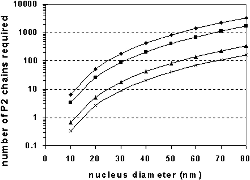
Number of second-stage (P2) polymer chains required to form nucleated domains for various molecular weights of P2. (♦) 50 000 g mol–1, (■) 100 000 g mol–1, (▴) 500 000 g mol–1, (×) 1 000 000 g mol–1.
To calculate the diffusion coefficient for a monomeric species, we have used the work published by Karlsson and al. [30]. We can calculate the polymer diffusion coefficient by using a simple scaling law for diffusion of polymer as presented by Piton et al. [31]:
| (20) |
| (21) |
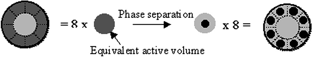
Illustrative representation of the equivalent volume accessible to polymerization. Diffusion over roughly half the diameter of the equivalent volume is necessary to achieve phase separation.
The number of separate nuclei that it is possible to form from a system at the spinodal composition is related to the conversion necessary to form one nucleus, X1, and the value of the spinodal composition for that particular system. Within these sub-volumes, the chains of polymer P2 have to travel on average half of the distance, in order to ‘meet’ at the center of the volume. Clearly some chains must diffuse a longer distance, and other a much smaller distance. The half distance assumption is both simplistic and reasonable for an average chain behavior. Consequently we can calculate the average distance that a chain needs to diffuse:
| (22) |
In order to appreciate whether a system is under going phase separation through nucleation and growth or spinodal decomposition, we need to compare the time it takes to produce a number of chains sufficient to create a domain with the time it takes for these chains to diffuse the necessary distance in order for them to assemble into a domain (tD). In a semi-continuous process, the time to polymerize one chain is the ratio of the total feed time over the number of chains constituting the second stage polymer. This time is given by:
| (23) |
| (24) |
Finally Eqs (14), (21), (22) and (24) can be combined to define a dimensionless ratio of the polymerization time, Tp, over diffusion time, tD, to yield Eq. (25):
| (25) |
Calculated times for polymerization and phase separation
| Experiment | A | B | C | D | D |
| → | Low conv. | High conv. | |||
| Feed time (s) | 34560 | 15600 | 15600 | 3600 | 3600 |
| Spinodal (v/v) | 0.01 | 0.01 | 0.01 | 0.02 | 0.01 |
| Wp (wt/wt) | 0.986 | 0.952 | 0.936 | 0.47 | 0.893 |
| FP | 0.11 | 0.41 | 0.13 | 1.0 | N/A |
| DN (nm) | 31 | 33 | 34 | 68 | 37 |
| D0 (nm) | 390 | 380 | 330 | 320 | 320 |
| a (nm) | 23 | 33 | 25 | 56 | 39 |
| DM (cm2 s–1) | 10–12 | 10–8 | 10–11 | 10–5 | 10–9 |
| tP (s) | 0.88 | 0.42 | 0.64 | 0.17 | 0.17 |
| nc/n | 18 | 21 | 23 | 174 | 30 |
| tD (s) | 8 × 10⁸ | 1 × 10⁵ | 6 × 10⁷ | 0.4 | 7 × 10⁵ |
| Tp/tD | 2 × 10⁻⁸ | 8 × 10⁻⁵ | 3 × 10⁻⁷ | 70 | 7 × 10⁻⁶ |
| Mechanism | SD | SD | SD | N&G | SD |
In the case of Experiment B we find that it takes 0.4 seconds to create a chain, that 21 chains are necessary to phase separate into a 33 nm nucleus, and that the time necessary for these chains to diffuse a distance of 33 nm to the nucleus location is 1 × 10⁵ seconds (30 hours). Clearly, phase separation cannot occur fast enough, and we would expect the system to enter the SD region. This ‘conclusion’ is justified by the low value of Tp/tD = 8 × 10⁻⁵. The situation is very similar for both Experiments A and C, with both having very small values of Tp/tD and thus these systems may also be expected to phase separate by spinodal decomposition.
In the case of Experiment D, which is the polymerization that was conducted in a batch manner, we see that the situation is quite different. At low conversion in this experiment the monomer concentration is very high and this leads to a diffusion coefficient for monomer of about 10–5 cm2 s–1 (which is almost irrespective of the Tg of the seed at this high monomer concentration). In this case, even though many more chains are required to form a single domain (174) and results in a much larger distance that the chains must diffuse over (56 nm), the time required for diffusion is much less than in the previous cases (0.4 s vs. many hours). It is seen that this faster diffusion rate results in the ratio Tp/tD now being significantly greater than 1, so that we would expect phase separation to occur by nucleation and growth in this case. However, when this batch experiment (D) is considered at high conversion, the situation is back to being one in which spinodal decomposition is more likely (Tp/tD is again much less than 1). This shows that in a case where the conditions within the latex particle may change significantly over the course of the reaction, such as in a batch reaction, the mechanism of phase separation may also change during the process.
Finally, it is noted that in all of the semibatch experiments presented in Table 5, it seems that phase separation may be more likely to occur by spinodal decomposition, while the only case that was likely to be nucleation and growth was the batch experiment. It should be pointed out that this is not a general rule and does not mean that all semibatch experiments phase separate by SD, or that all batch experiments undergo nucleation. In fact, it is quite possible to conceive of a situation in which a semibatch experiment would be more likely to phase separate by nucleation. Systems in which this would be likely are those in which the Tg of the seed polymer is substantially below the reaction temperature, which is a quite common situation in a latex polymerization. In this case, the diffusion coefficients will be relatively large, on the order of 10–5 to 10–6 cm2 s–1 for the value of DM, even though the monomer concentration in the semibatch experiment may be low. Other conditions that would tend to make nucleation more likely are small particle sizes and low molecular weights.
6 Conclusions
In this paper we have applied the nucleation and growth concepts to phase separation in latex particles to determine whether or not such computations can reasonably explain the phase structures we obtain from experiment. Indeed, such thermodynamic predictions for the critical nucleated domain size agree reasonably well with experiments. The distribution of domain sizes which develops over time is also fairly well predicted by considering the growth of the domains formed early in the process by polymerization reactions within those domains throughout the remainder of the process. Although it is a bit challenging to accurately measure the domain sizes in these particles, it does appear that the experimental conditions we used to prepare the latex particles via the semi-batch processes were adequate to preserve the phase separated structures throughout the polymerization process to allow direct comparison with predictions – i.e. we have no evidence of domain consolidation during reaction. On the other hand, phase consolidation, or ripening, is readily apparent in the results of the batch reaction. The NG calculations give us a potential new gauge for determining whether or not ripening has taken place. We conclude that composite latex particles that exist in their thermodynamic free-energy equilibrium state must have experienced phase consolidation in order to achieve that state.
Despite the agreement between the computed and experimental results, we are not convinced that phase separation in the semi-batch reactions has taken place via nucleation and growth. Several factors force us to consider the spinodal decomposition mechanism for phase separation in these experiments and this will be the subject of a future paper.
Acknowledgements
We are grateful for the use of the experimental results of Lina Karlsson, for the TEM images provided by Helen Hassander, and for critical discussions with Ola Karlsson, all of Lund University. We also appreciate the financial support provided by the UNH Latex Particle Morphology Industrial Consortium (AtoFina, Mitsubishi Chemicals, NeoResins and UCB Chemicals).