

1 Introduction
The extent and nature of the metal–metal (M–M) interactions in transition metal complexes where there are ligands which bridge the metal–metal bond has been of considerable interest and controversy [1,2]. Numerous theoretical studies, including ones on such proto-typical molecules as Fe2(CO)9 [2,3] or Co2(CO)8 [4] indicate that little direct metal–metal bonding is present in this situation, despite the requirement for a metal–metal bond from the 18-electron rule. Reflecting the importance of this topic, some of the first experimental charge density studies on organotransition metal complexes focussed on ligand-bridged M–M bonds [5–10]. These early studies utilised deformation density models to probe the nature of the M–M interaction, but this approach is not very suitable for these systems. The electron density ρ at the mid-point of the M–M internuclear vector is typically very small, ~0.1–0.2 e Å–3 for a single M–M bond, and it proved difficult to detect the expected charge concentrations. Moreover, these ambiguous results cast doubt on the ability of charge density studies to provide useful information concerning M–M interactions.
The atoms in molecules (AIM) approach of Bader [11] has become increasingly used in the analysis of experimental electron density. This topological method has the great advantage of avoiding the difficult choice of a suitable pro-density, and has been adopted in the experimental study of the M–M interactions in several transition metal carbonyl compounds [12–18]. The methodology provides an unambiguous definition of bonding between atoms [19] through the presence of (3, –1) critical points in the density ρ. These are points where the gradient of the density ∇(ρ) is zero and where the density is a minimum along the gradient path between two nuclei. They are commonly called bond critical points (bcp's). Moreover the AIM method also provides a rigorous quantum definition of the boundary between atoms, the so-called interatomic or zero-flux surface. At this surface, all vectors n normal to the surface are orthogonal to ∇(ρ), i.e. n·∇(ρ) = 0, and integration of the electron density inside this surface leads to a unique and non-arbitrary atomic charge partitioning.
The examination of properties such as the electron density ρ(rb), the Laplacian of ρ, i.e. ∇2ρ(rb) and also the kinetic energy density G(rb) and the total energy density H(rb) [i.e. G(rb) + V(rb)] at the (3, –1) bcp's leads to a classification of chemical bonds [11,20]. Shared or open shell (covalent) interactions, where the potential energy density V(rb) dominates over the kinetic energy density in the region of the interatomic surface, are characterised by large values of ρ(rb) and negative values of ∇2ρ(rb) and H(rb). Closed shell (ionic or van der Waals) interactions, where the kinetic energy density G(rb) dominates over the potential energy density in the region of the interatomic surface, are characterised by small values of ρ(rb), positive values of ∇2ρ(rb) and positive, near-zero values of H(rb). While these classifications are particularly useful for compounds of elements from the first and second periodic rows [11], they are less pertinent for transition metals. In a series of studies on M–M interactions in transition metal compounds containing bridging carbonyl ligands, Macchi et al. [1,14] have discussed the limitations of the above criteria. They also investigated a number of other useful criteria to characterise the M–M interactions, such as ∫A∩B ρ(rb), the integrated density over the interatomic surface separating two atoms and the delocalisation index δ(A, B) [21,22], a measure of the Fermi correlation shared between two atoms, i.e. a measure of the number of shared electrons.
Herein we report our experimental and theoretical charge density studies on Co3(μ3-CX)(CO)9 (1a X = H, 1b X = Cl). We focus on the nature of the M–M and M–CX interactions in these compounds, where the Co–Co vectors are bridged by an alkylidyne ligand μ3-CX, rather than by carbonyl groups. Compound 1a has been the subject of a previous charge density study by Coppens and Leung [23–25] using the deformation density methodology. This study is a good illustration of the problems of choosing suitable fragment pro-densities, since it appears [24,25] that the electron distribution in the μ3-CH ligand is intermediate between the 2Π ground state and the 4Σ excited state.
2 Experimental procedures
2.1 Data collection and processing
Compounds 1a and 1b were synthesised according to the literature methods [26]. Crystals suitable for data collection were obtained by sublimation at room temperature or recrystallisation from hexane. Details of data collection procedures are given in Table 1. Single crystals of suitable size were attached to glass fibres using silicone grease, and mounted on a goniometer head in a general position. They were cooled from ambient temperature over a period of 1 h, using an Oxford Instruments Cryostream. Data were collected on an Bruker–Nonius KappaCCD diffractometer, running under Nonius Collect software [27]. The Collect software calculates and optimises the goniometer and detector angular positions during data acquisition. The oscillation axis was either the diffractometer ω- or ϕ-axis with scan angles of 1–2°. Short scans were used to record the intense low-order data more accurately (absolute detector θ-offset for these scan-sets was < 7°). The scan-sets with low detector θ-offsets were measured first in the data collection strategy, to alleviate problems with ice-rings which gradually build-up during data collection. The high-angle images showed no evidence of contamination from ice-rings.
Experimental details
| Compound formula | C10HCo3O9 | C10ClCo3O9 |
| Compound colour | Black | Black |
| Mr | 441.90 | 476.34 |
| Space group | P–1 | P–1 |
| Crystal system | Triclinic | Triclinic |
| a (Å) | 7.9354(3) | 7.7993(2) |
| b (Å) | 13.6441(4) | 8.7214(2) |
| c (Å) | 6.8154(2) | 11.8259(3) |
| α (°) | 101.627(2) | 87.1640(10) |
| β (°) | 109.343(2) | 81.7130(10) |
| γ (°) | 93.942(2) | 67.6910(10) |
| V (Å3) | 674.60(4) | 736.42(3) |
| Z | 2 | 2 |
| Dcalc (g cm–3) | 2.175 | 2.148 |
| μ(Mo Kα) (mm–1) | 3.688 | 3.562 |
| Temperature (K) | 100(2) | 115(2) |
| θ Range (°) | 2.75–50.06 | 1.74–50.06 |
| Number of data used for merging | 184,003 | 218,448 |
| hkl range | –17 → 17; –29 → 29; –14 → 14 | –16 → 16; –18 → 18; –25 → 25 |
| Rint | 0.0291 | 0.0309 |
| Rσ | 0.0127 | 0.0140 |
| Spherical atom refinement | ||
| Number of data in refinement | 14,197 | 15,491 |
| Number of refined parameters | 204 | 209 |
| Final R [I > 2σ(I)] (all data) | 0.0176 (0.0195) | 0.0186 (0.0229) |
| Rw2 [I > 2σ(I)] (all data) | 0.0442 (0.0447) | 0.0470 (0.0482) |
| Goodness-of-fit S | 1.148 | 1.004 |
| Largest remaining feature in electron density map (e Å–3) | 0.714 (max) | 0.698 (max) |
| –0.684 (min) | –0.655 (min) | |
| Max shift/esd in last cycle | 0.001 | 0.004 |
| Multipole refinement | ||
| Number of data in refinement | 13,033 | 13,451 |
| Number of refined parameters | 584 | 642 |
| Final R [I > 3σ(I)] (all data) | 0.0116 (0.0150) | 0.0120 (0.0194) |
| Rw [I > 3σ(I)] | 0.0131 | 0.0116 |
| Goodness-of-fit S | 1.645 | 1.3751 |
| Largest remaining feature in electron density map (e Å–3) | 0.255 | 0.309 |
| –0.239 | –0.221 | |
| Max shift/esd in last cycle | 0.0002 | < 0.0001 |
The unit cell dimensions used for refinement purposes were determined by post-refinement of the setting angles of a significant portion of the data set, using the Scalepack program [28]. The cell errors obtained from this least-squares procedure are undoubtedly serious underestimates [29], but are used here in the absence of better estimates. The frame images were integrated using Denzo [23], and this is discussed in more detail in Section 2.4. The resultant raw intensity files from Denzo were processed using a locally modified version of DENZOX [30], which calculates direction cosines for the absorption correction, as well as applying rejection criteria on the basis of bad χ2 of profile-fit and ignoring partial reflections at the starting or final frame of a scan-set. Both data sets were truncated at sin(θ)/λ = 1.0788 (θmax = 50°), since the higher angle data were generally of low intensity and subject to integration errors due to the widening Kα1–α2 splitting. The resolution is sufficient to deconvolute the thermal parameters from the charge density effects, as gauged by the rigid-bond test (see Section 2.6).
An absorption correction by Gaussian quadrature [31], based on the measured crystal faces, was then applied to the reflection data. The data were then scaled using SADABS [32] to correct for any machine instabilities, and a semi-empirical absorption correction [33] (without a theta dependent correction) was applied to remove any residual absorption anisotropy due to the mounting medium. Batch scaling was also applied, with one scale factor per scan-set. No significant variations in scale factors were noted, indicating no sample decomposition. Data were sorted and merged using SORTAV [34].
2.2 Specific details for compound 1a
A total of 4614 frames from 68 scan-sets were measured over a time period of 151.3 h. An integration time of 6 s was used for scan-sets # 1–10, 60 s for scan-sets 11–36 and 168 s for the remaining scan-sets. A crystal of approximate size 0.41 × 0.39 × 0.33 mm was used and transmission coefficients were in the range 0.253–0.493. A total of 14,197 independent data were obtained after merging, with a mean redundancy of 13.0. The dataset is complete for 0 < θ ≤ 50.06°, apart from one missing low-order reflection (0 1 0). The data were then transformed to conform to the (non-standard) unit cell reported previously by Leung et al. [23].
2.3 Specific details for compound 1b
A total of 4582 frames from 79 scan-sets were measured over a time period of 152.6 h. Two crystals were used for data collection. The first 54 scan-sets were measured on a crystal of approximate dimensions 0.36 × 0.31 × 0.15 mm (range transmission coefficients 0.282–0.602), while a larger crystal of dimensions 0.56 × 0.47 × 0.12 mm (range transmission coefficients 0.185–0.653) was used for the remaining high-angle scans. Integration times were in the range 7–204 s per image. A total of 15,491 independent data were obtained after merging, with a mean redundancy of 14.1. The dataset has two high-order reflections missing in the range 0 < θ ≤ 50.06°.
2.4 Comparison of Denzo and EvalCCD integration
It has been recently commented in [35,36] that the Denzo program [28] is unsuitable for integration of high-resolution data, since explicit handling of the Kα1–α2 splitting is not included in the software. In order to examine this aspect of the data reduction, we have compared data integrated with Denzo with data obtained using the program EvalCCD [37], which utilises a completely different integration algorithm. Denzo refines a number of instrumental and crystal parameters, and a neighbourhood profile fitting [28] is used. The profile used for each individual spot is obtained from the profiles of other observed reflections in the vicinity in the same image. The profile is an averaged and normalised pixel-map, and it appears that the profile fitting used by Denzo provides an adequate allowance for any Kα1–α2 splitting. Supplementary Fig. S1 shows both a typical high-angle oscillation image displaying Kα1–α2 splitting, and the averaged profiles obtained by Denzo for that same image. The profiles are clearly elongated in the direction of the Kα1–α2 splitting. As a measure of the quality of integration, Denzo records a χ2 of profile-fit for each reflection. A plot of the averaged χ2 of profile-fit, averaged over small ranges of sin(θ)/λ, versus sin(θ)/λ is shown in Supplementary Fig. S2. This plot clearly indicates that there is no apparent problem with profile fitting of the high-angle data.
In EvalCCD [37], the impact of each diffraction event on the detector is calculated, assuming accurate instrumental calibration and others parameters such as crystal shape. Profile fitting is not used, but the program explicitly includes a correction factor for the Kα1–α2 splitting. The data were initially integrated with EvalCCD using an approximate orientation matrix obtained from the Denzo integration. The peak positions thus obtained provided a more accurate orientation matrix, which was then used to obtain the final integrated data. We find consistent differences between data integrated using the two programs. The I/σ(I) values for the most intense data are generally higher in the EvalCCD data, but for the weaker data this situation is reversed. Moreover in refinement, the R residuals are almost invariably higher for the EvalCCD data, especially those calculated using all data, and the electron density difference maps are noisier than those from the Denzo derived data. The ratio of IEval/IDenzo for individual reflections in the two suitably scaled data sets are shown in Fig. 1. It can be seen that over the range 0.75 < sin(θ)/λ < 1.1 there is no systematic trend, and the mean scale factor is quite constant. This indicates that there is no systematic problem in recovering the full intensities of the high-angle data using Denzo, or at least that both programs suffer similarly from any deficiency. There is a systematic difference of ~10% between the high- and low-angle ranges, which is not currently understood. It may arise from biases introduced in the averaging procedures due the differing standard uncertainties derived for individual measurement by the two programs. This systematic trend in scaling factors translates into the refined thermal parameters, which are uniformly lower when using the EvalCCD data. Overall we conclude that data obtained using Denzo are quite suitable for accurate charge density studies, and all the refinements discussed in this paper use these data.
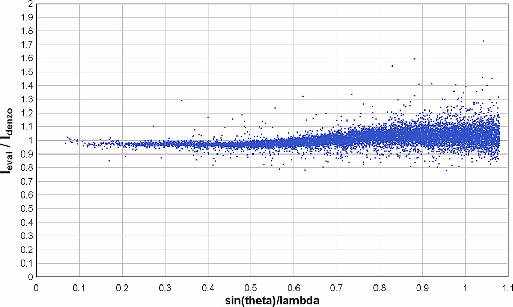
Scale factor between Eval and Denzo integrations for individual measurements in the data set of complex 1a as a function of sin(θ)/λ.
2.5 Spherical atom refinements
A spherical atom refinement using SHELXL97-2 [38] was initially undertaken, with full-matrix least-squares on F2 and using all the unique data. All non-H atoms were allowed anisotropic thermal motion. The H atom in 1a was included at the position observed in a difference map and freely refined. As expected, the X-ray refined C–H distance of 0.935(12) Å is shorter than the neutron determined [23] distance. A final difference maps shows the strongest remaining features in the region of the Co atoms, in patterns consistent with the crystal-field effects on the d-orbitals, i.e. negative peaks in the directions of the ligands. Neutral atom scattering factors, coefficients of anomalous dispersion and absorption coefficients were obtained from [39]. Details of this refinement are given in Table 1. Thermal ellipsoid plots (Figs. 3 and 4) were obtained using the program ORTEP-3 for Windows [40]. All calculations were carried out using the WinGX package [41] of crystallographic programs.
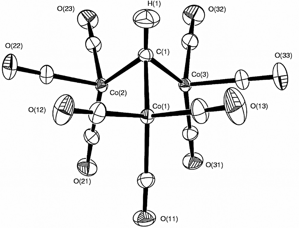
ORTEP plot of 1a (70% probability ellipsoids) from the multipole refinement, showing the atomic labelling scheme.
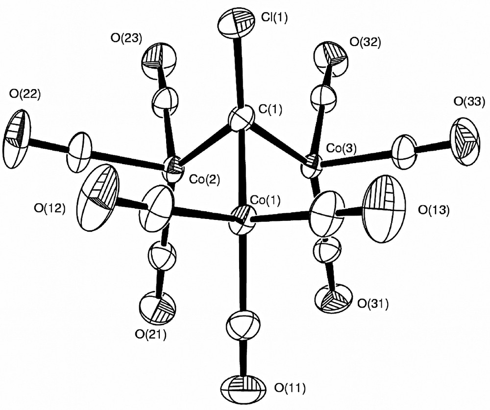
ORTEP plot of 1b (70% probability ellipsoids) from the multipole refinement, showing the atomic labelling scheme.
2.6 Multipole refinement
The valence density multipole formalism of Hansen and Coppens [42] as implemented in the XD program suite [43] was used. The function minimised in the least-squares procedure was Σw(|Fo| – k|Fc|)2, with only those reflections with I > 3σ(I) included in the refinement. The multipole expansion was truncated at the hexadecapole level for the Co and Cl atoms and at the octupole level for the C and O atoms. For the methylidyne hydrogen in 1a, a single bond-directed dipole was used. The hydrogen position was fixed at the neutron determined distance [23] of 1.084 Å, while the magnitudes of the anisotropic Uij tensor were taken from the same neutron diffraction study, scaled according to the procedure of Blessing [44] and kept fixed during refinement. Each pseudoatom was assigned a core and spherical-valence scattering factor derived from the relativistic Dirac–Fock wave-functions of Su and Coppens [45] expanded in terms of the single-ζ functions of Bunge et al. [46]. The radial fit of these functions was optimised by refinement of the expansion–contraction parameter κ. The valence deformation functions for the C, O and H atoms used a single-ζ Slater-type radial function multiplied by the density-normalised spherical harmonics. The radial fits for the chemically distinct C atoms (three types) and O atoms (two types) were optimised by refinement of their expansion–contraction parameters κ′, but models were also examined where these were fixed at the optimised values reported by Volkov et al. [47]. A number of different deformation density models were examined for the Co atoms. The radial terms used for the Co atoms were either simple Slater functions or the relevant order Fourier–Bessel transforms of the Su and Coppens [45] wave-functions. Attempts to refine the 4s population independently through the l = 0 deformation function (the second monopole) were unsuccessful; all such models proved unstable or gave physically unrealistic populations. The final model used the 4s23dn configuration, with the 4s electrons treated as core electrons. A single κ value was refined for each chemical type (1 Co, 2C, 1O), and an identical κ′ value refined for the l = 0–4 multipoles of the valence deformation. Final refined values are given in Supplementary Table S1. For the H atom in 1a, a fixed value of 1.0, 1.2 was used for κ and κ′, respectively. For the Cl atom in 1b, the κ′ value was kept fixed at 1.0, since refinement let to unrealistically contracted radial functions. Electro-neutrality constraints on the whole molecule were applied throughout refinements.
After a full multipole refinement using harmonic thermal motion for all atoms, the residual maps for 1a and 1b were essentially featureless, except in the vicinity of the Cl atom in 1b, where some sharp features are observed, see Fig. 2a and Supplementary Figs. S4 and S12. Recently Sørensen et al. [48] have reported difficulties in modelling the scattering of fluorine atoms in fluoro-aryl compounds, and attributed this to significant anharmonic thermal motion of the halogen. We have investigated for a similar effect in 1b. Refinement using third and fourth order Gram–Charlier expansions of the thermal parameter for the Cl atom led to the removal of these sharp features (Fig. 2b) and gave a significantly better fit. The final model for 1b therefore included anharmonic thermal motion of the Cl atom. The Hirshfeld rigid-bond criterion [49] is fulfilled in compound 1a for the C–O bonds (mean Δ-msda = 0.6 × 10⁻³ Å2), but the Co–C bonds slightly exceed the criterion (mean Δ-msda = 1.4 × 10⁻³ Å2). The Δ-msda for the C(1)–H(1) bond is 5.0 × 10⁻³ Å2, which indicates some deficiency in the scaled anisotropic displacement parameter (adp) for H(1), which was obtained from the previous neutron diffraction study [23]. For compound 1b the corresponding Δ-msda values are, respectively, 1.1 and 1.6 × 10⁻³ Å2. The worst individual Δ-msda value is 2.6 × 10⁻³ Å2 for C(11)–O(11). Scatter-plots of the scale factor between observed and final calculated F as a function of sin(θ)/λ display no significant trends (Supplementary Fig. S3).
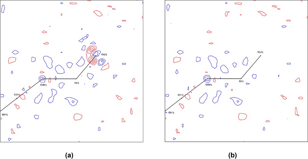
Residual maps (Fobs – Fmulti) for complex 1b through the plane Co(1)–C(1)–Cl(1) (a) prior to introduction of anharmonic thermal motion for Cl(1) and (b) after inclusion of third and fourth order Gram–Charlier coefficients on Cl(1). Positive contours are drawn in blue, negative contours in red, at intervals of 0.1 e Å–3.
The kinetic energy densities at the bcp's G(r) for the experimental densities given in Table 3 were estimated using the approximation of Abramov [50]:
Summary of topological properties at bcp's in compounds 1a and 1b a
| ρ(rb) b | ∇2ρ(rb) c | ɛ | G(rb) d,e | V(rb) d | H(rb) d | |
| Co–C(1) | 0.789(6) | 7.796(9) | 0.08 | 0.91 | –1.26 | –0.36 |
| 0.850 | 6.241 | 0.016 | 0.751 | –1.065 | –0.314 | |
| 0.843(6) | 7.830(8) | 0.14 | 0.97 | –1.39 | –0.42 | |
| 0.854 | 6.721 | 0.016 | 0.780 | –1.089 | –0.309 | |
| C(1)–X | 1.791(32) | –17.585(99) | 0.02 | 1.30 | –3.84 | –2.53 |
| 1.896 | –23.154 | 0.00 | 0.255 | –2.131 | –1.876 | |
| 1.380(12) | –3.731(20) | 0.04 | 1.20 | –2.66 | –1.46 | |
| 1.377 | –7.007 | 0.00 | 0.515 | –1.520 | –1.005 | |
| Co–C(ax) | 0.887(8) | 11.891(15) | 0.11 | 1.21 | –1.59 | –0.38 |
| 0.864 | 12.970 | 0.045 | 1.178 | –1.448 | –0.270 | |
| 0.940(7) | 10.939(11) | 0.07 | 1.24 | –1.70 | –0.47 | |
| 0.865 | 13.043 | 0.048 | 1.184 | –1.455 | –0.271 | |
| Co–C(eq) | 0.965(9) | 13.035(18) | 0.05 | 1.37 | –1.82 | –0.46 |
| 0.944 | 13.704 | 0.013 | 1.286 | –1.613 | –0.327 | |
| 0.982(7) | 11.638(12) | 0.06 | 1.32 | –1.83 | –0.51 | |
| 0.931 | 13.639 | 0.018 | 1.271 | –1.588 | –0.316 | |
| C–O(ax) | 3.425(24) | –8.259(213) | 0.04 | 5.88 | –12.32 | –6.45 |
| 3.229 | 13.659 | 0.001 | 6.648 | –12.339 | –5.692 | |
| 3.320(22) | 4.584(199) | 0.03 | 6.15 | –11.99 | –5.83 | |
| 3.225 | 13.501 | 0.001 | 6.627 | –12.309 | –5.682 | |
| C–O(eq) | 3.350(26) | –15.935(226) | 0.04 | 5.29 | –11.69 | –6.40 |
| 3.221 | 13.366 | 0.001 | 6.617 | –12.298 | –5.681 | |
| 3.312(25) | –4.383(215) | 0.05 | 5.72 | –11.74 | –6.02 | |
| 3.238 | 13.980 | 0.001 | 6.699 | –12.420 | –5.721 |
a Top line gives experimental values for 1a, second line gives theoretical values from DFT calculations for 1a, third and fourth lines, the corresponding values for 1b.
b In units of e Å–3.
c In units of e Å–5.
d In units of Hartree Å–3.
e Estimated by the approximation of Abramov [50].
2.7 Theoretical studies
Single-point SCF calculations on 1a and 1b at the experimental geometry of the isolated molecule (symmetrised to C3v) were performed, using the DFT option in the GAMESS-UK program suite [51]. Basis sets were obtained from EMSL1. To ascertain any basis set dependency, the topological properties were examined with a minimal basis 3-21G, with a 6-31G basis, and finally a 6-311G** basis for C, O, H, Cl and the Wachters basis with additional f polarisation functions for Co [52,53]. The B3LYP functional [54] was used throughout. The overall topology and molecular graph showed no basis set dependence. Atomic properties were obtained from the theoretical densities using a locally modified version of the AIMPAC programs [55] or AIM2000 [56]. Critical points in the Laplacian function, L(r), ≡ –∇2ρ(r), in the i-VSCC of the Co atoms were searched using the BUBBLE algorithm [57], for both the theoretical and experimental densities.
3 Results and discussion
3.1 Description of the structures
The atomic labelling schemes and thermal ellipsoids for 1a and 1b are shown in Figs. 3 and 4. The X-ray crystal structure of complex 1b [58] and a combined X-ray and neutron diffraction study on 1a [23] have been previously reported, and Table 2 give a comparison of important metrical parameters for 1a and 1b from this study and these previous studies. The agreement between studies is excellent, with differences generally below 3σ. The structural features of the Co3(μ-CX)(CO)9 moiety are, of course, very well established, with more than 120 examples in the Cambridge Crystallographic Data Base. The values of bond distances and angles reported in Table 2 are well within the ranges found. The mean values in the data base are Co–Co = 2.47(1), Co–Calkylidyne = 1.90(3) and Co–Ccarbonyl = 1.79(4) Å.
Important bond distances (Å) and bond angles (°) for 1a and 1b
| 1a a | 1a b | 1a c | 1b a | 1b d | |
| Bonds | |||||
| Co(1)–Co(2) | 2.47665(11) | 2.480(2) | 2.4769(6) | 2.47674(19) | 2.476(1) |
| Co(1)–Co(3) | 2.48752(11) | 2.486(2) | 2.4886(5) | 2.48237(18) | 2.488(1) |
| Co(2)–Co(3) | 2.47321(11) | 2.476(2) | 2.4729(5) | 2.47288(18) | 2.477(2) |
| Co(1)–C(1) | 1.8918(3) | 1.893(1) | 1.892(2) | 1.8893(3) | 1.892(6) |
| Co(2)–C(1) | 1.8934(3) | 1.895(1) | 1.889(2) | 1.8963(3) | 1.897(7) |
| Co(3)–C(1) | 1.8953(3) | 1.897(1) | 1.894(2) | 1.8822(3) | 1.885(7) |
| Co(1)–C(11) | 1.8388(4) | 1.838(1) | 1.835(2) | 1.8309(4) | 1.798 |
| Co(1)–C(12) | 1.7931(4) | 1.796(1) | 1.794(2) | 1.8052(4) | 1.797 |
| Co(1)–C(13) | 1.7976(4) | 1.798(2) | 1.797(2) | 1.8076(4) | 1.768 |
| Co(2)–C(21) | 1.8411(3) | 1.842(1) | 1.841(2) | 1.8338(4) | 1.796 |
| Co(2)–C(22) | 1.7981(4) | 1.799(1) | 1.799(2) | 1.7991(4) | 1.789 |
| Co(2)–C(23) | 1.8003(3) | 1.800(2) | 1.801(2) | 1.7953(4) | 1.797 |
| Co(3)–C(31) | 1.8301(4) | 1.832(1) | 1.835(2) | 1.8413(3) | 1.820 |
| Co(3)–C(32) | 1.7998(4) | 1.801(1) | 1.797(2) | 1.8063(4) | 1.828 |
| Co(3)–C(33) | 1.7898(3) | 1.792(2) | 1.789(2) | 1.8036(4) | 1.820 |
| C(1)–X e | 1.084 f | 1.084(1) | 0.94(2) | 1.7167(3) | 1.707 |
| C(11)–O(11) | 1.1369(7) | 1.136(1) | 1.137(3) | 1.1426(10) | 1.163 |
| C(12)–O(12) | 1.1408(8) | 1.137(1) | 1.140(3) | 1.1396(10) | 1.136 |
| C(13)–O(13) | 1.1428(9) | 1.135(1) | 1.133(3) | 1.1435(11) | 1.149 |
| C(21)–O(21) | 1.1374(7) | 1.136(1) | 1.134(2) | 1.1423(9) | 1.158 |
| C(22)–O(22) | 1.1401(7) | 1.137(1) | 1.138(3) | 1.1425(9) | 1.134 |
| C(23)–O(23) | 1.1411(7) | 1.138(1) | 1.134(2) | 1.1368(8) | 1.145 |
| C(31)–O(31) | 1.1388(7) | 1.137(1) | 1.131(2) | 1.1390(8) | 1.157 |
| C(32)–O(32) | 1.1402(8) | 1.138(1) | 1.137(3) | 1.1377(8) | 1.111 |
| C(33)–O(33) | 1.1432(7) | 1.138(1) | 1.137(3) | 1.1333(9) | 1.157 |
| Angles | |||||
| Co(1)–C(1)–X e | 131.21(2) | 131.41 | – | 130.180(18) | 130.24 |
| Co(2)–C(1)–X e | 130.56(2) | 131.21 | – | 129.598(18) | 129.77 |
| Co(3)–C(1)–X e | 130.90(2) | 130.29 | – | 132.555(19) | 132.16 |
| Co(1)–C(1)–Co(2) | 81.734(11) | 81.79 | – | 81.725(13) | 81.80 |
| Co(1)–C(1)–Co(3) | 82.120(12) | 82.04 | – | 82.323(13) | 82.46 |
| Co(2)–C(1)–Co(3) | 81.505(11) | 81.59 | – | 81.755(12) | 81.81 |
| Co(1)–Co(2)–Co(3) | 60.337(3) | 60.21 | – | 60.202(5) | 60.3 |
| Co(2)–Co(1)–Co(3) | 59.763(3) | 59.81 | – | 59.822(5) | 59.9 |
| Co(1)–Co(3)–Co(2) | 59.900(3) | 59.97 | – | 59.976(5) | 59.8 |
| Cax–Co–C(1) av. | 142.43 | 142.41 | – | 141.95 | 142.08 |
| Ceq–Co–C(1) av. | 101.67 | 101.68 | – | 102.11 | 102.41 |
The Co–Calkylidyne distances are somewhat shorter than expected2 for a Co–C(sp3) interaction, and are consistent with some multiple bond character. The mean Co–C(1) distance in 1a is 1.8935 Å and in 1b is marginally shorter at 1.8891 Å, possibly reflecting a greater π-acidity of the μ3-CCl group. As previously noted [23], in both 1a and 1b, the axial carbonyl ligands, trans to the Co-alkylidyne vector, are quite distinct from the equatorial ligands. The mean Co–Cax distance in 1a and 1b is 1.837 and 1.835 Å, respectively, while the corresponding mean Co–Ceq distances are 1.796 and 1.803 Å, respectively. In compound 1a, the axial C–O distances are also systematically smaller than the equatorial C–O distances (mean values are 1.137 and 1.141 Å, respectively), but this trend is not mirrored in 1b. The ν(CO) IR stretching frequencies are ~5 cm–1 higher for 1b compared with 1a [59], suggesting that the μ3-CCl group is a poorer σ-donor/better π-acceptor than the μ3-CH group, which is expected based on the relative electronegativities of Cl and H.
3.2 Topological analysis
Static and dynamic model maps, experimental deformation maps, residual maps and Laplacian (–∇2ρ) maps through the tri-cobalt plane and the three Co–C–X planes are shown in Supplementary Figs. S4–S20. These maps show the expected charge build-up in the C–O, Co–C and C–X bonds, but no such corresponding build-up along the Co–Co vectors. The results of topological analyses of the experimental and theoretical charge densities in both 1a and 1b are summarised in Table 3, and full details are given in Supplementary Tables S3 and S4. The expected (3, –1) bcp were found for all covalent bonds, except for the Co–Co interactions, and the molecular graph derived from the experimental charge density for 1a is shown in Fig. 5. The qualitative features of this molecular graph are quite reproducible, and depend neither on the exact multipole model used for the experimental analysis, nor on the basis sets or molecular coordinates used in the deriving the calculated densities. The agreement between the experimental and theoretical values of the topological descriptors is quite reasonable, especially for 1a. In most cases the experimental values for ρ(rb) are slightly higher than the theoretical values. The major disagreement concerns the Laplacian values for the C–O bonds in the carbonyls, which is a well understood issue [1,18] related to the fact that the bcp lies close to the nodal plane. For all the Co–C bonds, the value of ∇2ρ(rb) is positive, though ρ(rb) is significantly above zero. As argued previously [1,18], the negative value for the total energy density H(rb) for these bonds implies that these interactions should be considered as open shell (covalent) interactions. The C–X bonds have the “classic” open shell topological properties, with a large value for ρ(rb), a negative value for ∇2ρ(rb) and a significantly negative H(rb).
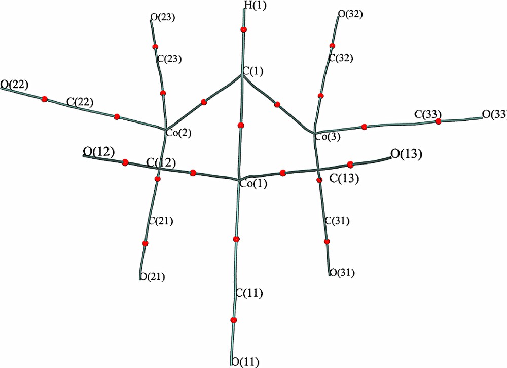
Molecular graph for 1a taken from the experimental charge density. Labels indicate the atomic positions and spheres indicate the (3, –1) bcp's.
In line with the Co–C distances associated with the carbonyl ligands, the value of ρ(rb) for the Co–C(eq) bonds are significantly greater than for the Co–C(ax) bonds. Moreover the values of ρ(rb) for the Co–CX bonds are smaller still, suggesting that the bond orders for the Co–C bonds follow the sequence Co–C(eq) > Co–C(ax) > Co–CX. The topological properties associated with the M–C–O bonds are very similar to those reported in numerous other studies [1,12–18] and merit little further comment. The nature of the Co–Calkylidyne bond is discussed further in Section 3.4.
3.3 The nature of the Co–Co interactions
A major point of interest is the complete lack of any (3, –1) bcp's between the cobalt atoms. Within the AIM paradigm, the presence of a bcp is taken a universal indicator of chemical bonding [19], so we are forced to conclude that there is no direct bonding interaction between the cobalt atoms. In a closely related study, Macchi and Sironi [1] have followed the evolution in the topological properties of M–M and M–CO interactions as a CO ligand is translated towards a triply-bridging geometry in the hypothetical anion [Co3(μ3-CO)(CO)9]–. It was found that the M–M bond path disappears quite early along the reaction coordinate, at a Co–Cbridging distance of ~2.2 Å, and the lack of such a bond path in compounds like 1, with symmetric μ3-CR ligands, is therefore not surprising. Evidently many of the conclusions regarding bridging CO ligands [1] may be extended to alkylidyne ligands. There is an interesting difference however, in that Macchi and Sironi [1] report inwardly curved bond paths from the μ3-CO ligand to the Co atoms, whereas in compound 1 the bond paths from the μ3-CR ligand are quite linear (see Fig. 5). This is an indication of the localisation of the Co–Calkylidyne interaction (see below).
It is tempting to conclude that strong ligand-bridging interactions always ‘destroy’ the topological M–M bond. A bcp between the metal atoms is always found in those cases where there is an unsupported M–M interaction, e.g., in Mn2(CO)10 [15,18] or Co2(CO)6(AsPh3)2 [12]. However, whereas there are many examples of ligand-bridged M–M bonds which have ring structures lacking a bcp [4,13,14,60,61], this is by no means a universal finding. In experimental studies by Bianchi et al. [16,17] on Co2(CO)6(μ-CO)(μ-C4O2H2) and also in theoretical studies, e.g., on Co2(μ-NO)2Cp2 [60], Ni2(μ-InMe)2Cp2 [62] and [Mo3(μ2-S)3(μ3-S)Cl3(PH3)6]+ [63], bcp's have been observed between strongly ligand-bridged metal atoms. The presence or otherwise of a bcp may also be highly dependent on geometry, as was found for Co2(μ-NO)2Cp2 [60]. These ambiguities are undoubtedly related to the difficulty of defining the topology of the density in regions of very flat density, such as found in M–M interactions, where λ2 is close to zero.
The lack of a bcp between the Co atoms severely limits the interpretation of any Co–Co interaction within the AIM paradigm. The presence of significant Co–Co interactions in compound 1 has been reported from Extended Hückel or Fenske–Hall MO studies [64–66], and we sought further evidence for these. The delocalisation index δ(A, B) [21,22] is one AIM indicator of chemical bonding between atoms which does not rely on the presence of a bcp. As mentioned in Section 1, this index provides a measure of the electrons shared between two atoms. The delocalisation index is easily computable from a single configurational wave-function, but cannot be obtained from the experimental density. At the Hartree–Fock level, δ(A, B) is in good agreement with Lewis theory [22], and for M–M bonds it has been shown [1] to be rather insensitive to the nature of bridging interactions. The values of δ(A, B) obtained for 1a and 1b are given in Table 5. The magnitude of δ(Co, Co) is 0.47, which is quite substantial and is in fact identical to that computed by Macchi and Sironi [1] for the Co–Co bond in the unbridged form of Co2(CO)8, which possesses a direct Co–Co bond. This indicates there is a substantial Co–Co interaction in 1, albeit probably indirect and mainly mediated by the bridging alkylidyne group. The significance, within the AIM paradigm, of inter-atomic interactions which result in large delocalisation indices, but no bond paths is not yet clear. The delocalisation indices associated with the 1,3 Co···C interactions are quite small, but when combined may make a significant contribution towards the M–M interaction [1].
Delocalisation indices δ(A, B)
| A, B | 1a | 1b |
| Co, Co | 0.47 | 0.47 |
| Co, Calk | 0.89 | 0.86 |
| Co, Ceq | 1.00 | 0.99 |
| Co, Cax | 0.95 | 0.93 |
| Co, Oeq | 0.16 | 0.16 |
| Co, Oax | 0.14 | 0.14 |
| C, O (eq) | 1.63 | 1.64 |
| C, O (ax) | 1.65 | 1.65 |
The molecular graph shown in Fig. 5 suggests that the coordination geometry of the Co atoms could be considered as tetrahedral, but the atomic graphs of these atoms, in both the theoretical and experimental densities are clearly octahedral. The theoretical derived atomic graph of the Co atom in 1a is shown in Fig. 6, together with an isosurface plot of the experimental Laplacian for Co(2) in 1a. The atomic graph [11] defines the topology of the three types of critical points in –∇2ρ found in the valence shell charge concentration (VSCC) of an atom. This topology describes the distortions in the valence shell of an atom on chemical bonding, and the (3, –3) charge concentrations may be associated with bonding and non-bonding electron pairs of the Lewis formalism. The atomic graph shown in Fig. 6 is characteristic of octahedral transition metals, for example for the Mn atom in Mn2(CO)10 [18]. The six (3, +1) charge depletions face the positions of the six ligands, while the eight (3, –3) charge concentrations occupy the faces of an octahedron, maximally avoiding the ligand positions. In complex 1, the three carbonyl ligands directly face charge depletions, while the two Co–Co vectors are also closely aligned with charge depletions. This is clearly seen in Fig. 6b, which also shows that the Co-μ3–CH vector is quite misaligned from the corresponding charge depletion. If the Co–Co vectors are included in the coordination sphere of a cobalt atom, it may be considered as a significantly distorted octahedron. It is interesting to note that this distortion is not manifest in the atomic graph of the Co atom, which appears to adopt a quite undistorted octahedral topology.
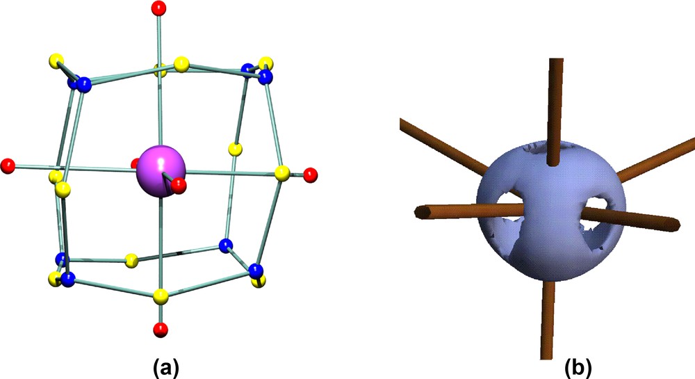
(a) Theoretical atomic graph of the Co atom in compound 1a. The critical points in the Laplacian L ≡ –∇2ρ in the VSCC are colour coded as (3, –3) blue, (3, –1) yellow, (3, +1) red. (b) Isosurface plot of the experimental L (at +750 e Å–5) for the Co(2) atom in complex 1a. The view is along the bisector of the Co(1)–Co(2) and Co(2)–Co(3) bonds, with the Co(2)–C(1) vector vertical.
3.4 The nature of the Co3–C(alkylidyne) interaction
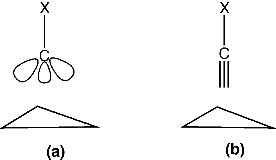
Previous MO studies on 1 [64–66] have discussed the bonding of the μ3-CX ligand to the Co3 cluster in terms either of a localised sp3 bonding (A) or a delocalised sp type bonding (B). The consensus was that the latter description (B) was most appropriate. In a previous charge density study on 1a by Leung and Coppens [24,25], the charge density in the μ3-CH group was analysed in terms of the 2Π ground state and the 4Σ excited state of this ligand. These two states correspond approximately to B and A, respectively, and the deformation densities indicated that both states were involved in the bonding.
We note two points of relevance concerning the geometric parameters of C(1):
- • The geometry at the alkylidyne carbon C(1) is a strongly distorted tetrahedron, see Table 2, but is rather similar in 1a and 1b.
- • The Co–C(1) distances are significantly shorter than expected for a Co–C(sp3) bond, but are longer than the Co–C(carbonyl) distances.
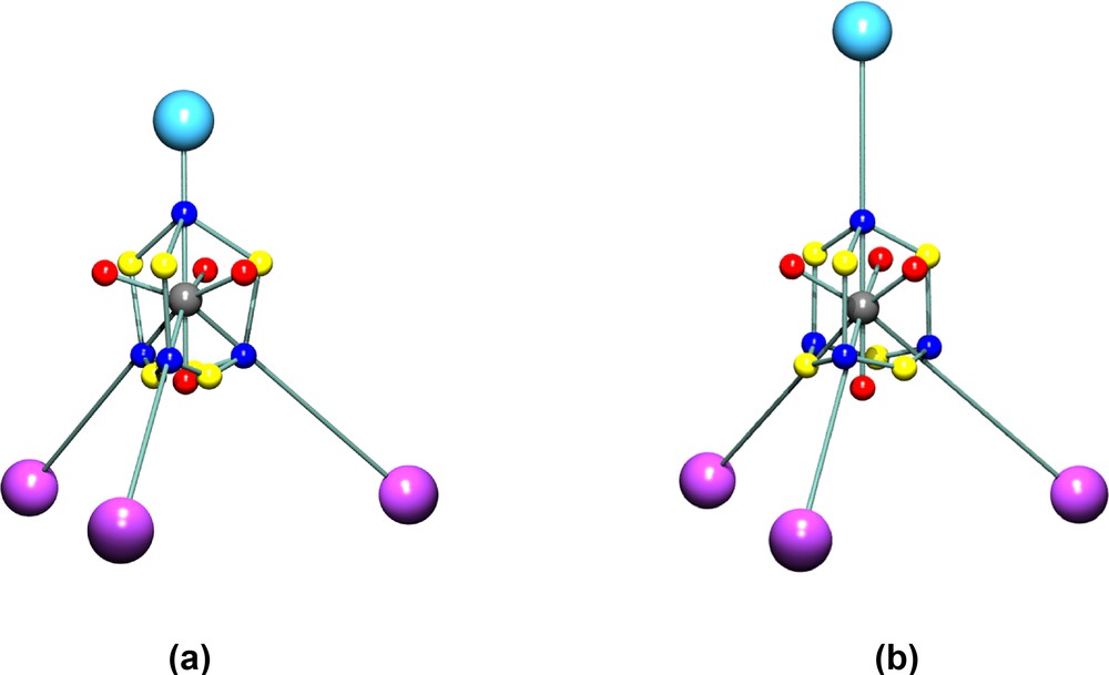
Schematic atomic graph of the alkylidyne carbon atom C(1) in (a) compound 1a and (b) in compound 1b. The critical points in L ≡ –∇2ρ in the VSCC of C(1) are colour coded as (3, –3) blue, (3, –1) yellow, (3, +1) red. The positions of the Co and H/Cl atoms are indicated by purple and pale blue spheres, respectively.
The localisation of the VSCCs appears more pronounced in the chloro compound 1b than in 1a. The charge concentrations directed towards the Co atoms are virtually identical in both complexes, but the charge concentration facing the Cl atom in 1b is much reduced compared with that facing the H atom in 1a, see Table S2. This is due to the greater electronegativity of Cl compared with H. These differing localisations are also obvious from the isosurfaces of the Laplacian function –∇2ρ, shown in Fig. 8, and the contour plots shown in Fig. 9. The latter clearly show the excellent agreement between experimental and theoretical results. The greater overall polarisation in the VSCC of C(1) in 1b towards the X atom is understandable in view of the greater electronegativity of the Cl atom versus H. The model deformation maps shown in Fig. 10 also clearly show the greater localisation in 1b and may be compared with the deformation maps reported by Leung and Coppens [24,25].
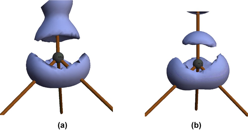
Isosurface plots of the experimental Laplacian L ≡ –∇2ρ (at +10 e Å–5) for the atom C(1) in complex 1a (a) and complex 1b (b). The vertical vector shows the direction of the X atom of the CX group.
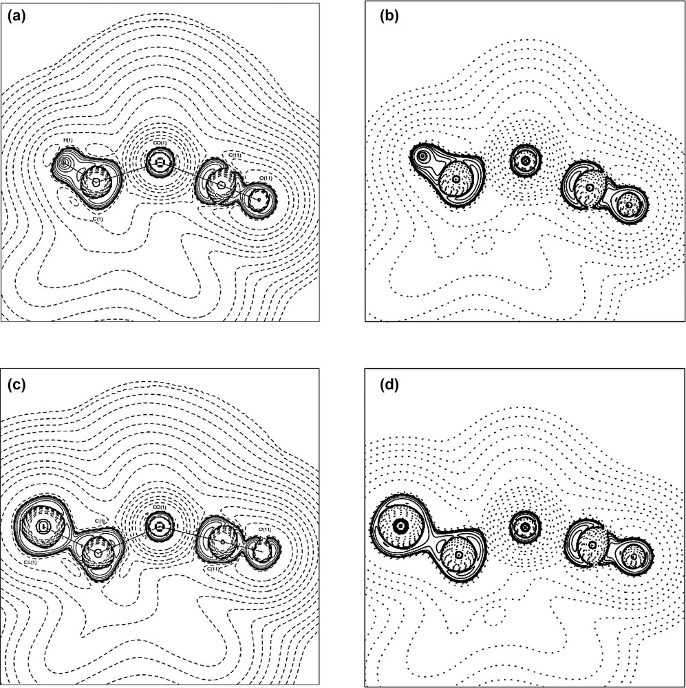
Contour plots of the Laplacian L ≡ –∇2ρ through the Co(1)–C(1)–X plane in complex 1a (a), (b) and complex 1b (c), (d). The experimental results are shown in (a), (c) and the theoretical results in (b), (d). Contours are drawn at ±2.0 × 10n, ±4 × 10n, ±8 × 10n (n = –3, –2, –1, 0, +1) e Å–5.
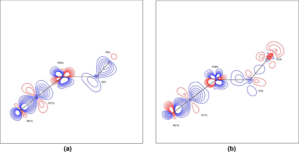
Static model deformation maps (ρmulti – ρsph) for complex 1a (a) and complex 1b (b) through the plane Co(1)–C(1)–X. Positive contours are drawn in blue, negative contours in red, at intervals of 0.1 e Å–3.
3.5 Atomic charges
The atomic charges from the experimental and theoretical studies, derived by a variety of methods, are given in Table 4. The atomic charge is a concept of fundamental interest to chemists, but has proved difficult to quantify accurately. In part this arises because of the problem of experimentally measuring such charges [68]. Meister and Schwartz [69] have demonstrated that the scale of the derived charges can differ by a factor of ~10, depending on the chosen method. The AIM charges, obtained by numerical integration over the volume enclosed by the zero-flux surface of each atom (the atomic basin) have been shown [70] to be relatively insensitive to the choice of basis set, but generally lead to larger atomic charges than other methods. In this study it can be seen that there is good agreement between the experimental and theoretical AIM charges. Most methods agree in assignment of a positive charge to the Co atoms and a negative charge to the alkylidyne carbon C(1). For other atoms there is less agreement, for instance the multipole derived charges q(Pv) for the carbonyl C and O atoms are even of opposite sign to those obtained from other methods. Apart from the lower experimental value of q(Ω) for 1b, all methods agree in assigning a greater negative overall charge for the CX group in 1b, consistent with the view that the μ3-CCl group is a poorer σ-donor/better π-acceptor than the μ3-CH group.
Atomic charges
| Atom | 1a | 1b | ||||||
| q(Pv) a | q(Ω) b | q c | q(Ω) d | q(Pv) a | q(Ω) b | q c | q(Ω) d | |
| Co(1) | 0.090 | 0.619 | 0.324 | 0.536 | 0.127 | 0.446 | 0.203 | 0.539 |
| Co(2) | 0.112 | 0.636 | 0.324 | 0.536 | 0.090 | 0.434 | 0.203 | 0.540 |
| Co(3) | 0.114 | 0.624 | 0.324 | 0.536 | 0.119 | 0.449 | 0.203 | 0.540 |
| C(1) | –0.108 | –0.478 | –0.373 | –0.505 | –0.368 | –0.132 | –0.660 | –0.356 |
| Caxial | –0.152 | 0.866 | 0.239 | 0.976 | –0.257 | 0.845 | 0.233 | 0.974 |
| Cequatorial | –0.148 | 0.977 | 0.304 | 1.001 | –0.204 | 1.012 | 0.307 | 1.010 |
| Oaxial | 0.104 | –1.044 | –0.144 | –1.122 | 0.180 | –1.091 | –0.144 | –1.120 |
| Oequatorial | 0.157 | –1.092 | –0.147 | –1.116 | 0.246 | –1.027 | –0.142 | –1.113 |
| X e | –0.121 | 0.020 | 0.122 | 0.035 | 0.004 | –0.251 | 0.010 | –0.190 |
| Sum CX | –0.229 | –0.458 | –0.251 | –0.470 | –0.364 | –0.383 | –0.650 | –0.546 |
a Multipole populations experimental study.
b AIM charges experimental study.
c Mulliken populations DFT calculation.
d AIM charges DFT calculation.
e X = H(1) in 1a and Cl(1) in 1b.
3.6 Thermal motion analyses
The thermal motion in 1a and 1b has been analysed in terms of the TLS formalism [71], and the full results are given in Table S5. For 1a, the hydrogen atom was not included in the analysis, due to the deficiency in the adp mentioned above. The whole molecule of 1a was initially treated as a rigid body. The resultant libration tensor T was approximately isotropic, with an rms value ~2°, indicating there was no significant preferential rigid body librational motion. The large value of 0.112 for wR, which is the discrepancy index between observed and calculated adps, is indicative of some additional internal motion. The PEANUT [72] plots shown in Fig. 11 display the rmsd surface (90% probability) for the difference between the calculated and observed adp's. From Fig. 11a, it is clear that the oxygen atoms of the equatorial carbonyls in particular show excess motion, mainly normal to the equatorial plane. In view of the well known fluxional motion associated with a tripodal rotation of M(CO)3 groups, the inclusion of independent Co(CO)3 tripodal librations for each group was investigated. While the wR value was reduced to 0.084, it is clear that this does not account well for the excess thermal motion, as can be seen in Fig. 11b. Complex 1b shows broadly similar behaviour (Fig. S21).
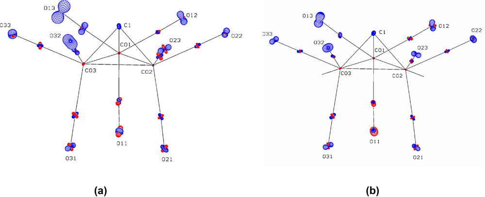
PEANUT plots for complex 1a showing the rmsd difference (90% probability) between observed and calculated adp's for (a) a pure rigid body motion and (b) a rigid body motion coupled with independent Co(CO)3 tripodal librations. Positive differences are drawn in blue, negative differences in red. The adp for the H atom was not included in the calculation.
4 Conclusion
The AIM analysis on the charge densities in Co3(μ3-CX)(CO)9 (1a X = H, 1b X = Cl) shows unambiguously that there are no (3, –1) bcps between the Co atoms, and hence no direct Co–Co bonding is observable. However, the delocalisation indices δ(Co, Co) indicate significant electron pair sharing between Co centres, which must be mediated by the bridging alkylidyne ligand. The topology of the Laplacian in the VSCC of the alkylidyne carbon is homeomorphic with that of methane, so that significant Co–C bond localisation must be present. The geometrical and density parameters are consistent with a small degree of bond multiplicity and hence π-bonding between the Co3 triangle and the alkylidyne ligand.
5 Supplementary materials
Supplementary material in the form of CIF files (spherical atom and multipole refinements) have been deposited with deposition numbers CCDC 236121–236124. These data can be obtained free of charge via www.ccdc.cam.ac.uk/data_request/cif, by emailing data_request@ccdc.cam.ac.uk, or by contacting The Cambridge Crystallographic Data Centre, 12, Union Road, Cambridge CB2 1EZ, UK; fax: +44 1223 336033. Additional supplementary materials consisting of structure factor listings (CIF format), Supplementary Figs. (S1–S21) and Supplementary Tables (S1–S9) are available from the author on request.
Acknowledgements
We thank the EPSRC for grant GR/M91433 towards the purchase of a KappaCCD diffractometer and for access to the Columbus DEC 8400 Superscalar Service (RAL). The New Zealand Foundation for Research, Science and Technology is thanked for financial (PDRA) support for C.E. We also thank Professor Piero Macchi (Milano) for many helpful discussions.
1 Basis sets were obtained from the Extensible Computational Chemistry Environment Basis Set Database, Version 12/03/03, as developed and distributed by the Molecular Science Computing Facility, Environmental and Molecular Sciences Laboratory which is part of the Pacific Northwest Laboratory, P.O. Box 999, Richland, Washington 99352, USA, and funded by the U.S. Department of Energy. The Pacific Northwest Laboratory is a multi-program laboratory operated by Battelle Memorial Institute for the U.S. Department of Energy under contract DE-AC06-76RLO 1830. Contact David Feller or Karen Schuchardt for further information.
2 The mean Co–C(sp3) distance in the 19 complexes in the Cambridge Crystallographic Data Base containing the (CO)3Co–C(sp3) fragment is 2.09(3) Å.