Modeling properties of molecules with open d-shells using density functional theory

Mihail Atanasov; Claude A. Daul

doi:10.1016/j.crci.2005.04.003

Account / Revue

Modeling properties of molecules with open d-shells using density functional theory

Mihail Atanasov ^1,² ; Claude A. Daul ¹

¹ Département de Chimie, université de Fribourg, chemin du Musée 9, CH-1700 Fribourg, Switzerland
² Institute of General and Inorganic Chemistry, Bulgarian Academy of Sciences, 1113 Sofia, Bulgaria

Comptes Rendus. Chimie, Volume 8 (2005) no. 9-10, pp. 1421-1433.

Résumés

Anglais
Français

An overview of the theory and applications of a recently proposed ligand-field density functional theory (LFDFT) is given. We describe a procedure based on DFT allowing to deduce the parameters of this non-empirical LF approach consisting of the following steps: (i) an average of configuration (AOC) DFT calculation, with equal occupancies of the d-orbitals is carried out (ii) with these orbitals kept frozen, the energies of all single determinants (SD) within the whole LF-manifold are calculated and used as a data base in a further step to provide all the Racah- and LF-parameters needed in a conventional LF-calculation. A more rigorous analysis of this approach in terms of Löwdin's energy partitioning and effective Hamiltonians is used to provide explicit context for its applicability and to set more rigorous criteria for its limitations. The formalism has been extended to account for spin-orbit coupling as well. Selected applications cover tetrahedral CrX₄ (X = Cl, Br) and FeO₄^2– and octahedral CrX₆^3– (X = F^–, Cl^–, Br^–) complexes. Transition energies are calculated with an accuracy of 2000 cm^–1, deviations being larger for spin-forbidden transitions and smaller for spin-allowed ones. Analysis show, that ligand field parameters deduced from experiment are well reproduced, while interelectronic repulsion parameters are calculated systematically to be by 30–50% of lower in energy. A generalization of the LFDFT theory to dimers of transition metals allows to calculate exchange coupling integrals in reasonable agreement with experiment and with comparable success to the broken symmetry approach; in addition they allow to judge ferromagnetic contributions to exchange coupling integral which have been ignored before. .

Une vue d'ensemble est apportée ici sur la théorie et les applications de la récente théorie des fonctionnelles de la densité du champ de ligand (LFDFT). Nous décrivons une procédure basée sur la théorie de la fonctionnelle de la densité (DFT), permettant de déduire les paramètres de cette approche non empirique du champ de ligand, comprenant les étapes suivantes : (i) un calcul DFT de configuration moyenne (AOC) est effectué, avec une occupation égale des orbitales d, (ii) avec ces orbitales figées, les énergies de tous les déterminants simples (SD) dans l'espace du champ de ligand sont calculées et sont utilisées comme base de données lors de l'étape suivante, pour fournir tous les paramètres Racah et champ de ligand nécessaires dans un calcul classique de champ de ligand. Une approche plus rigoureuse en termes de partition d'énergie selon Löwdin et d'hamiltonien effectif est utilisée pour fournir un contexte explicite à son applicabilité et pour mettre en place des critères plus rigoureux, dans le but de fixer les limites de la méthode. Le formalisme est étendu pour prendre aussi en compte le couplage spin–orbite. Les exemples sélectionnées comprennent les complexes tétrahédriques CrX₄ (X = Cl, Br) et FeO₄^3– (X = F^–, Cl^–, Br^–). Les énergies de transition sont calculées avec une précision de ±2000 cm^–1, les déviations étant plus grandes pour les transitions de spin interdites et plus petites pour celles qui sont autorisées. L'analyse montre que les paramètres de champ de ligand déduits de l'expérimentation sont bien reproduits, tandis que les paramètres de répulsion inter-électronique sont calculés systématiquement de 10 à 20% plus petits. Une généralisation de la théorie de la fonctionnelle de densité du champ de ligand aux dimères des métaux de transition permet de calculer les constantes de couplage d'échange en accord raisonable avec l'expérimentation et avec un succès comparable à l'approche de la symétrie brisée ; de plus, ils permettent de juger des contributions du ferromagnétisme à la constante de couplage d'échange, qui jusqu'à présent avait été ignorée. .

Métadonnées

Reçu le : 2004-05-13
Accepté le : 2005-04-28
Publié le : 2005-08-08

DOI : 10.1016/j.crci.2005.04.003

Keywords: Density functional theory, Ligand-field theory, Spin–orbit coupling, Zero-field splitting, Magnetic exchange coupling
Mots clés : Théorie de la fonctionnelle de la densité, Théorie du champ de ligand, Couplage spin–orbite, Zero-field splitting, Couplage d'échange magnétique

Affiliations des auteurs :

Mihail Atanasov ^{1, 2} ; Claude A. Daul ¹

@article{CRCHIM_2005__8_9-10_1421_0,
     author = {Mihail Atanasov and Claude A. Daul},
     title = {Modeling properties of molecules with open d-shells using density functional theory},
     journal = {Comptes Rendus. Chimie},
     pages = {1421--1433},
     publisher = {Elsevier},
     volume = {8},
     number = {9-10},
     year = {2005},
     doi = {10.1016/j.crci.2005.04.003},
     language = {en},
}

TY  - JOUR
AU  - Mihail Atanasov
AU  - Claude A. Daul
TI  - Modeling properties of molecules with open d-shells using density functional theory
JO  - Comptes Rendus. Chimie
PY  - 2005
SP  - 1421
EP  - 1433
VL  - 8
IS  - 9-10
PB  - Elsevier
DO  - 10.1016/j.crci.2005.04.003
LA  - en
ID  - CRCHIM_2005__8_9-10_1421_0
ER  -

%0 Journal Article
%A Mihail Atanasov
%A Claude A. Daul
%T Modeling properties of molecules with open d-shells using density functional theory
%J Comptes Rendus. Chimie
%D 2005
%P 1421-1433
%V 8
%N 9-10
%I Elsevier
%R 10.1016/j.crci.2005.04.003
%G en
%F CRCHIM_2005__8_9-10_1421_0

Mihail Atanasov; Claude A. Daul. Modeling properties of molecules with open d-shells using density functional theory. Comptes Rendus. Chimie, Volume 8 (2005) no. 9-10, pp. 1421-1433. doi : 10.1016/j.crci.2005.04.003. https://comptes-rendus.academie-sciences.fr/chimie/articles/10.1016/j.crci.2005.04.003/

Version originale du texte intégral

1 Introduction

When describing electronic structures of transition metal complexes one goes a different way from the point of view of quantum chemistry and experimental spectroscopy. Experimentalists make use of ligand field parameterized (effective) Hamiltonians, or of the spin-Hamiltonian when interpreting optical or ESR spectra, or they apply the Heisenberg exchange operator in the case of magnetic exchange coupling. Empirical models of that kind have been therefore tools for description, rather than tools for prediction of ligand field properties. A quantum chemist solves more or less rigorously numerically the Schrödinger equation (ab initio) or the Kohn–Sham equations (density functional theory, DFT) and is able to make predictions as well. However, numerical results are sometimes not easy to interpret or analyze and the bridge between the ab-initio approach and chemical intuition is not always transparent. DFT became increasingly popular in recent time. As manifested by the groups of Baerends, Ziegler [1,2] and Daul [3] it is able to predict both ground and excited states of TM complexes. Recently, a new approach has been developed in our group [4]. It is based on a multi-determinant description of the multiplet structure originating from the well defined dⁿ configurations of a TM in the surrounding of coordinating ligands by combining the CI and the DFT approaches. In doing so, both dynamical (via the DFT exchange-correlation potential) and non-dynamical (via CI) correlation is introduced, the latter accounting for the rather localized character of the d-electron wavefunction. The key feature of this approach is the explicit treatment of near degeneracy effects (long-range correlation) using ad hoc configuration interaction (CI) within the active space of Kohn–Sham (KS) orbitals with dominant d-character. The calculation of the CI-matrices is based on a symmetry decomposition and/or on a ligand field analysis of the energies of all single determinants (SD, micro-states) calculated according to DFT for frozen KS-orbitals corresponding to the averaged configuration, eventually with fractional occupations of the d-orbitals. This procedure yields multiplet energies with an accuracy within 2000 cm^–1. Currently, the procedure has been extended to spin-orbit coupling [5] and allows to also treat Zero-Field Splitting (ZFS) [6], Zeeman interactions and Hyper-Fine Splitting (HFS) [7] and magnetic exchange coupling [8] as well.

In this account a more rigorous analysis of our approach utilizing Löwdin's energy partitioning [9] and effective Hamiltonians theory [10,11] is used, providing explicit context for its applicability and allowing to set up more rigorous criteria for its limitations. We will then briefly sketch the mathematical procedure behind our approach. An extension to spin-orbit coupling will be also given. Selected applications cover tetrahedral CrX₄ (X = Cl, Br) and FeO₄^2– and octahedral CrX₆^3–(X = F^–, Cl^–, Br^–) complexes. In addition the spin-orbit coupling constant of Cr(acac)₃ deduced from a DFT-ZORA calculation will be applied to calculate the ground and excited state zero-field splitting.

A generalization of the LFDFT theory to dimers of transition metals allows to calculate exchange coupling integrals in reasonable agreement with experiment and with comparable success to the broken symmetry approach; in addition they allow to judge ferromagnetic contributions to exchange coupling integrals, the latter are usually being ignored. An illustration of how the procedure works will be given for hydroxo-dimers of Cu²⁺.

2 Partitioning technique, effective Hamiltonians and the ligand field approach

Let us consider a system consisting of transition metals and ligands, which can be bridging or terminal (Fig. 1). In electronic structure calculations, one usually immediately recognizes antibonding molecular orbitals (MO's), as being dominated by metal |nd〉 functions, which are partly filled and bonding orbitals dominated by ligand AO's which are fully occupied. Following Löwdin [9] we can write down the Schrödinger equation H ψ = E ψ in a discrete representation based on the use of a complete orthonormal set Φ = {Φ_k} and introduce the Hamiltonian matrix H = $[\begin{matrix} ... & ... & ... \\ ... & {\begin{matrix} H \end{matrix}}_{k l} & ... \\ ... & ... & ... \end{matrix}]$ and the column vector c = $[{c_{k}}_{...}^{...}]$ using the relations:(1)

H_{k l} = 〈 Φ_{k} | H | Φ_{l} 〉, c_{k} = 〈 Φ_{k} | Ψ 〉

(2)

Ψ = \sum_{k} c_{k} Φ_{k}

(3)

H c = E c

Fig. 1
Partioning scheme for LFDFT approach of a pair of transition metals joined by bridging ligands.

Let us subdivide the system into two parts, one build of from metal nd-orbitals (d) and another composed of valence metal (n + 1) s and (n + 1) p and ligand functions (v).

Then the eigenvalue problem (3) can be represented in a form given by:(4)

[\begin{matrix} {\begin{matrix} H \end{matrix}}_{{d d}^{'}} & {\begin{matrix} H \end{matrix}}_{d v} \\ {\begin{matrix} H \end{matrix}}_{v d} & {\begin{matrix} H \end{matrix}}_{{v v}^{'}} \end{matrix}] \begin{matrix} [\begin{matrix} {\vec{\begin{matrix} c \end{matrix}}}_{d} \\ {\vec{\begin{matrix} c \end{matrix}}}_{d} \end{matrix}] = [\begin{matrix} {\begin{matrix} E 1 \end{matrix}}_{d} & 0 \\ 0 & {\begin{matrix} E 1 \end{matrix}}_{v} \end{matrix}] \end{matrix} [\begin{matrix} {\vec{\begin{matrix} c \end{matrix}}}_{d} \\ {\vec{\begin{matrix} c \end{matrix}}}_{v} \end{matrix}] = E [\begin{matrix} {\begin{matrix} 1 \end{matrix}}_{d} & 0 \\ 0 & {\begin{matrix} 1 \end{matrix}}_{v} \end{matrix}] [\begin{matrix} {\vec{\begin{matrix} c \end{matrix}}}_{d} \\ {\vec{\begin{matrix} c \end{matrix}}}_{v} \end{matrix}]

with 1_d and 1_v the identity matrices of dimension N_d × N_d and N_v × N_v, respectively.

Collecting terms with same dimension, we get:(5.1)

[H_{d d} - E 1_{d d}] {\vec{c}}_{d} + H_{d v} {\vec{c}}_{v} = \vec{0}

(5.2)

H_{v d} {\vec{c}}_{d} + [H_{v v ′} - E 1_{v}] {\vec{c}}_{v} = \vec{0}

One can easily express the column vector ${\vec{c}}_{v}$ in terms of ${\vec{c}}_{d}$ (Eq. (6)), and after substitution into Eq. (5.1), one obtains a Hamiltonian completely restricted to the d-subspace:(6)

{\vec{c}}_{v} = {(H_{v v ′} - E 1_{v})}^{- 1} H_{v d} {\vec{c}}_{d}

(7)

(H_{d d ′} - E I_{d}) {\vec{c}}_{d} + H_{d v} {(H_{v v ′} - E I_{v})}^{- 1} H_{v d} {\vec{c}}_{d} = \vec{0}

We thus arrive at a pseudo-eigenvalue equation (Eq. (8)), with the explicit form of $H_{d d ′}^{′}$ given by Eq. (9). No approximation is inherent in Eq. (9). The representation given by Eq. (9) provides:(8)

H_{d d ′}^{′} {\vec{c}}_{d} = E I_{d} {\vec{c}}_{d}

(9)

H_{d d ′}^{′} = H_{d d ′} + H_{d v} {(H_{v v ′} - E I_{v})}^{- 1} H_{v d}

the physical background of ligand-field theory. The matrix H_dd´ represents the purely electrostatic effect of the metal d-orbitals by the surrounding ligand nuclei and the valence electron distribution excluding the d-electrons. It is subject of the usual description in terms of a ‘crystal-field theory’ applied to TM impurities in crystals. Since orbitals of the subsystems d and v are orthogonal to each other, the H_dd´ matrix also incorporates important exchange (Pauli) repulsion terms; these have been shown to be proportional to the squares of corresponding overlap integrals, allowing one to formulate the ligand field as a pseudopotential [12]. The second term in Eq. (9) is energy dependent. For diagonal

H_{d d ′}^{′}

, perturbation expansions (which presuppose |H_vv – H_dd|>> |H_vd|) allow us to identify E with the corresponding diagonal element of H_dd´. It is this second term that reflects metal–ligand covalency (charge-transfer) and is the subject of parameterization by the angular overlap model (AOM) [13,14]. Earlier analysis based on Eq. (9) have been purely theoretical, attempting to place a correct context and limits of applicability of ligand-field approach within the main body of quantum chemistry [15]. In Section 3, we describe a practical scheme allowing to deduce the matrix H_dd´ from DFT and to apply it directly to the calculation of dⁿ electronic multiplets.

The one-electron representation of Eq. (9) can easily be extended to systems with more than one TM. The $H_{d d ′}^{′}$ matrix for such cases contains terms that account for d-electron delocalization (via the second term in Eq. (9)) from one metal to another – indirect (via the bridging ligands) or direct (via corresponding off-diagonal terms of H_dd´) [15]. It gives rise to magnetic exchange coupling. This will be the topic of Section 4.

Finally, the one-electron scheme given by Eq. (9) can be extended to the many electron states resulting from the redistribution of all the d-electrons within the active d-orbital subspace. Their treatment requires two-electron repulsion integrals in addition to the one-electron ones. The general scheme we describe in Section 3 allows to also deduce these intergrals from DFT.

3 The ligand-field density functional theory (LFDFT)

The current DFT software includes functionals at the Local Density Approximation (LDA) and Generalized Gradient Approximation (GGA) levels. The former approximation is well adapted for molecular structure calculation: M–L bond lengths are usually accurate to ±0.02 Å but bond energies are too large. The latter approximation, however, is roughly twice as expensive in computer time and yields M–L bond energies accurate to ±5 kcal mol^–1. Recently a new generation of functionals called meta-GGA emerged. These functionals are more accurate but also more expensive and their implementation in computer codes is not yet generalized. It is generally accepted that all these functionals (LDA and GGA) describe well the so-called dynamical correlation, however, none of them includes near degeneracy correlation. In the method described next we address this problem specifically and include CI of valence electrons on the d-orbitals. The calculation scheme we developed includes three steps as described next.

We assume that we know the molecular geometry, either from a first principle geometry optimization or from X-ray data. Moreover, for the sake of simplicity, let us focus the following description to open d-shells: the extension to open f-shells is similar. The first step consists in a spin-restricted, i.e. same orbitals for same spin, Self-Consistent Field (SCF) DFT calculation of the average of the dⁿ configuration (AOC), providing an equal occupation n/5 on each MO dominated by the d-orbitals. The KS-orbitals which we construct using this AOC are best suited for a treatment in which, interelectronic repulsion is – as is done in LF theory, approximated by atomic-like Racah parameters B and C. The next step consists in a spin-unrestricted calculation of the manifold of all Slater Determinants (SD) originating from the dⁿ shell, i.e. 45, 120, 210 and 252 SD for d^2,8, d^3,7, d^4,6, and d⁵ Transition Metal (TM) ions, respectively. These SD-energies are used in the third step to extract the parameters of the one-electron 5 × 5 LF matrix $d_{μ} | h_{L F} | d_{v}$ as well as Racah's parameters B and C in a procedure, which we describe below. Finally, we introduce these parameters as input for a LF program allowing to calculate all the multiplets using CI of the full LF-manifold utilizing the symmetry as much as possible. We should note that in classical LF theory, it is only the LF matrix which carries information about the symmetry and the actual bonding in the complex, thus providing useful chemical information.

In order to establish a link between ligand field theory and the energy of each SD mentioned earlier we need to introduce an effective LF-Hamiltonian $h_{L F}^{e f f}$ together with its five eigenfunctions φ_i ${h_{L F}^{e f f} φ_{1} = ɛ_{i} φ_{i}, i = 1,...,5}$ which are in general linear combination of the five d-orbitals:(10)

[\begin{matrix} φ_{1} \\ φ_{2} \\ φ_{3} \\ φ_{4} \\ φ_{5} \end{matrix}] = C \cdot [\begin{matrix} {\begin{matrix} d \end{matrix}}_{x y} \\ \begin{matrix} {\begin{matrix} \begin{matrix} d \end{matrix} \end{matrix}}_{x z} \\ \begin{matrix} {\begin{matrix} \begin{matrix} d \end{matrix} \end{matrix}}_{y z} \\ \begin{matrix} {\begin{matrix} \begin{matrix} d \end{matrix} \end{matrix}}_{x^{2} - y^{2}} \\ d_{z^{2}} \end{matrix} \end{matrix} \end{matrix} \end{matrix}]

and where C is an orthogonal 5 × 5 matrix. Using this definition we can express the energy of each SD in terms of

〈 φ_{i} | h_{L F}^{e f f} | φ_{i} 〉

, the diagonal elements of the ligand-field splitting operator and electrostatic Coulomb and exchange integrals:(11)

\begin{array}{l} E ({SD}_{k}^{φ}) = E (\det | φ_{i (k,1)} σ_{i (k,1)} φ_{i (k,2)} σ_{i (k,2)} ... φ_{i (k, n)} σ_{i (k, n)} |) \\ = E_{0} + \sum_{i \in k} 〈 φ_{i} | h_{L F}^{e f f} | φ_{i} 〉 + \sum_{i < j} (J_{i j} - K_{i j} δ_{σ_{i} σ_{j}}) \end{array}

The SD $_{k}^{φ}$ are labeled with the subscript k = 1, …, $(\begin{matrix} 10 \\ \begin{matrix} - \\ \begin{matrix} \begin{matrix} n \end{matrix} \\ - \end{matrix} \end{matrix} \end{matrix})$ and where the superscript φ does refer to eigenfunctions of the ligand-field Hamiltonian h_LF. The summation i ∈ k of ligand-field splitting matrix elements $〈 φ_{i} | h_{L F}^{e f f} | φ_{i} 〉$ specify the occupation of the level φ_i, while $J_{i j} = 〈 φ_{i} φ_{i} | φ_{j} φ_{j} 〉$ and $K_{i j} = 〈 φ_{i} φ_{j} | φ_{i} φ_{j} 〉$ denote Coulomb and exchange integrals; σ_i are spin functions and E₀ represents the gauge origin of energy. This expression does only involve $〈 φ_{i} | h_{L F}^{e f f} | φ_{i} 〉$ the diagonal matrix elements of $h_{L F}^{e f f}$ . In order to obtain $〈 d_{μ} | h_{L F}^{e f f} | d_{ν} 〉$ , the full matrix representation of $h_{L F}^{e f f}$ , we make use of the general observation that the KS-orbitals and the set of SD considered in Eq. (11) convey all the information needed to setup the LF matrix. In Ref. [4], we give a justification for this.

Thus, let us denote KS-orbitals dominated by d-functions which result from an AOC dⁿ DFT-SCF calculation with a column vectors $\vec{V_{i}}$ . From the components of the eigenvector matrix build up from such columns one takes only the components corresponding to the d functions. Let us denote the square matrix composed of these column vectors by U and introduce the overlap matrix S:(12)

{S = U U}^{T}

Since U is in general not orthogonal, we use Löwdin's symmetric orthogonalization scheme to obtain an equivalent set of orthogonal eigenvectors (C):(13)

C = S^{- \frac{1}{2}} U

We identify now these vectors as the eigenfunctions of the effective LF-Hamiltonian $h_{L F}^{e f f}$ , we seek as(14)

φ_{i} = \sum_{μ = 1}^{5} c_{μ i} d_{μ}

Thus, the fitting procedure described below will enable us to estimate $h_{i i} = 〈 φ_{i} | h_{L F}^{e f f} | φ_{i} 〉 =$ and hence the full representation matrix of $h_{L F}^{e f f}$ as(15)

h_{μ ν} = 〈 d_{μ} | h_{L F}^{e f f} | d_{v} 〉 = \sum_{i = 1}^{5} c_{μ i} h_{i i} c_{v i}

In order to calculate the electrostatic contribution (second term in Eq. (11)), it is useful to consider the transformation from the basis of

S D_{k}^{φ}

to the one of

S D_{μ}^{d}

. Using basic linear algebra, we get:(16)

| S D_{k}^{φ} 〉 = \sum_{μ} T_{k μ} | S D_{μ}^{d} 〉

where

T_{k μ} = d e t | c_{i (k, l : n), j (μ, l : n)} |

i.e. the determinant of a n × n sub-matrix of

C \otimes σ

_, i.e. the direct product between C and

[\begin{matrix} 1 & 0 \\ 0 & 1 \end{matrix}]

:(17)

| \begin{matrix} c_{i (k, 1), j (µ, 1)} & c_{i (k, 1), j (µ, 2)} & ... & c_{i (k, 1 : n), j (µ, n)} \\ c_{i (k, 2), j (µ, 1)} & c_{i (k, 2), j (µ, 2)} & ... & c_{i (k, 2), j (µ, n)} \\ [\begin{matrix} \begin{matrix} ... \end{matrix} \end{matrix}] & [\begin{matrix} \begin{matrix} ... \end{matrix} \end{matrix}] & \begin{matrix} ... \end{matrix} & [\begin{matrix} \begin{matrix} ... \end{matrix} \end{matrix}] \\ c_{i (k, n), j (µ, 1)} & c_{i (k, n), j (µ, 2)} & c_{i (k, n), j (µ, n)} \end{matrix} |

with the indices of the spin orbitals

φ_{i (k, 1)} σ_{i (k, 1)}, φ_{i (k, 2)} σ_{i (k, 2)},..., φ_{i (k, n)} σ_{i (k, n)}

and

d_{j (μ, 1)} σ_{j (μ, 1)}, d_{j (μ, 2)} σ_{j (μ, 2)},..., d_{j (μ, n)} σ_{j (μ, n)}

, respectively. Note that these indices are in fact a two-dimensional array of (number of SD) × (number of electrons or holes) integers. Finally, the energy of a SD in Eq. (11) can be rewritten as:(18)

E_{k} = E (S D_{k}^{φ}) = \sum_{i} 〈 φ_{i} | h_{L F} | φ_{i} 〉 + \sum_{μ, ν} T_{k μ} T_{k ν} 〈 S D_{μ}^{d} | G | S D_{ν}^{d} 〉

where G = 1/r₁₂, i.e. the electrostatic repulsion of all electron pairs in the LF manifold. The matrix elements in the second term of Eq. (18) are readily obtained using Slater's rules and the resulting electrostatic two-electron integrals < ab|cd > in terms of Racah's parameters.

$\vec{X} = {(h}_{11},..., h_{55},B,C)$ Having obtained energy expressions for each ${SD}_{k}^{φ}$ : $〈 φ_{i} | h_{L F} | φ_{i} 〉$ , B, C and E₀ are estimated using a least-square procedure. Using matrix notation, we obtain an overdetermined system of linear Eq. (19), with the unknown parameters stored in and given by:(19)

\vec{E} = A \vec{X}

(20)

\vec{X} = {(A^{T} A)}^{- 1} A^{T} \vec{E}

It is worthwhile to note that the KS-eigenvalues $ɛ_{i}^{}$ of the orbitals with dominant d character are almost equal to the ligand-field parameters obtained in the fitting procedure, i.e.:(21)

ɛ_{i}^{KS} ≅ E_{0} + 〈 φ_{i} | {h_{L F}}_{} | φ_{i} 〉

Thus, we conclude this section with the statement that the separation between KS-eigenvalues of orbitals with dominant d-character are good approximations for the ligand field splitting parameters.

For cases where the fine-structure is sought it is now easy to include spin–orbit coupling and calculate:(22)

〈 {SD}_{k}^{d} | ζ_{d} \sum_{i = 1}^{n} ℓ_{i} ⋅ s_{i} | {SD}_{k'}^{d} 〉

where ζ_d is the spin–orbit coupling constant, whose value is easily obtained either from a ZORA [16] calculation [5] or from the radial part of the d-orbitals as:(23)

〈 d_{μ} | ζ (\vec{r}) | d_{ν} 〉 \approx k_{o r b_r e d} 〈 R_{n d} | r^{- 3} | R_{n d} 〉

where k_{orb_red} is an orbital reduction factor equal to the population on the metal Ao's. Thus, properties involving spin–orbit coupling are obtained in adding (22) to the full LF-Hamiltonian H₀ + H_{ligand field} + H_{elect_rep} + H_spin–orbit and calculating the sought properties from its eigenfunctions.

From the splitting (due to the combined effect of spin-orbit splitting and perturbations of symmetry lower than O_h), say of the ³A₂ and ⁴A₂ of hexa-coordinate ground states of Ni(II), d⁸ and Cr(III), d³, it is possible to obtain the ZFS D-tensor using a conventional spin-Hamiltonian approach:(24)

H_{Z F S} = \vec{S} \cdot D \cdot \vec{S} = D ({\hat{S}}_{z}^{2} - \frac{2}{3}) + E ({\hat{S}}_{x}^{2} - {\hat{S}}_{y}^{2})

and equating the energies of the spin–orbit components of the ³A₂ or ⁴A₂ to the eigenvalues of this spin Hamiltonian. An application of this approach is presented in Section 6.3.

4 LFDFT and magnetic exchange coupling

The approach of Section 3 has been extended to the calculation of the exchange coupling constant of Heisenberg Hamiltonian (Eq. (25)) in the case of pairs of TM joined by bridging ligands [8]. Taking a TM pair with S₁ = S₂ = 1/2 spins, the singlet–triplet separation is given by Eq. (26), implying a positive and negative values of J₁₂ for ferromagnetic and antiferromagnetic constants, respectively:(25)

H_{S} = - J_{12} S_{1} . S_{2}

(26)

E_{S = 0} - E_{S = 1} = J_{12}

Let us assume that two semi-occupied orbitals l₁ and l₂ on M₁ and M₂ couple to yield an in-phase (a) and an out-of-phase (b) MO (Eq. (27)).(27)

\begin{array}{l} a = \frac{1}{\sqrt{2}} (d l_{1} + d l_{2}) \\ b = \frac{1}{\sqrt{2}} (d l_{1} - d l_{2}) \end{array}

Six micro-states or SD are possible. Two are doubly occupied $| a^{+} a^{-} |$ , $| b^{+} b^{-} |$ and four are singly occupied $| a^{+} b^{-} |$ , $| a^{+} b^{+} |$ , $| a^{-} b^{+} |$ , $| a^{-} b^{-} |$ . The doubly occupied SD correspond to closed shells and are spin singlets, whereas the singly occupied SD correspond to a singlet and to a triplet. The two SD with M_S = 0: $| a^{+} b^{-} |$ and $| a^{-} b^{+} |$ , are mixed states belonging to a singlet and to a triplet. The energies of all these determinants can be easily calculated from DFT. Let us denote their energies, respectively, by:(28)

E_{1} = E (| a^{+} a^{-} |),

E_{2} = E (| b^{+} b^{-} |),

E_{3} = E (| a^{+} b^{+} |) = E (| a^{-} b^{-} |),

E_{4} = E (| a^{+} b^{-} |) = E (| a^{-} b^{+} |),

To obtain these energies, a two-step calculation scheme is applied. First a spin-restricted calculation with a so-called average of configuration (AOC) occupation (…a¹b¹) is carried out yielding a corresponding set of MOs {… a, b, …}. In a second step, these Kohn–Sham orbitals are kept frozen in order to evaluate the four SD-energies E₁, E₂, E₃ and E₄ (spin-polarized DFT) without further SCF iterations. We note that the E₄ – E₃ difference equals the exchange integral [ab|ab] which is also the quantity accounting for the mixing (1:1 in the limit of a full localization) between the a⁺a^– and b⁺b^– functions. This leads to matrix (Eq. (29)) which after diagonalization yields the eigenvalues E_– and E₊ and the singlet-triplet energy separation E_– – E₃, i.e. J₁₂:(29)

[\begin{matrix} E_{1} & (E_{4} - E_{3}) \\ (E_{4} - E_{3}) & E_{2} \end{matrix}]

Within the Anderson exchange model [17], dl₁ and dl₂ are singly occupied in the ground state giving rise to a triplet and a singlet with wave functions ψ_T and ψ_S (Eqs. (30, 31)). There are two further singlet states $ψ_{S}^{C T}$ and $ψ_{S}^{' C T}$ arising when either of the two magnetic electrons is transferred to the other magnetic orbital, i.e.:(30)

ψ_{T} = | d l_{1}^{+} d l_{2}^{+} |; | d l_{1}^{-} d l_{2}^{-} |; \frac{1}{\sqrt{2}} (| d l_{1}^{+} d l_{2}^{-} | + | d l_{1}^{-} d l_{2}^{+} |);

(31)

\begin{array}{l} ψ_{S} = \frac{1}{\sqrt{2}} (| d l_{1}^{+} d l_{2}^{-} | - | d l_{1}^{-} d l_{2}^{+} |) \\ ψ_{S}^{C T} = \frac{1}{\sqrt{2}} (| d l_{1}^{+} d l_{1}^{-} | + | d l_{2}^{+} d l_{2}^{-} |); ψ_{S}^{′ C T} = \frac{1}{\sqrt{2}} (| d l_{1}^{+} d l_{1}^{-} | - | d l_{2}^{+} d l_{2}^{-} |); \end{array}

with ψ_S being by 2 K₁₂ higher in energy than ψ_T. We take the energy of the latter state as reference {E(ψ_T) = 0}. K₁₂ is the classical Heisenberg exchange integral (Eq. (32)):(32)

K_{12} = \iint d l_{1} {(1)}^{*} d l_{2} (1) \frac{1}{r_{12}} d l_{1} {(2)}^{*} d l_{2} (2) d V_{1} d V_{2} = [d l_{1} d l_{2} | d l_{1} d l_{2}]

which is always positive. It reflects the exchange stabilization of the triplet over the singlet due to gain in potential energy connected with the spatial extension of the Fermi (exchange) hole (potential exchange). The ψ_S function can mix with the charge transfer state

ψ_{S}^{CT}

. Its energy, denoted with U equals the difference between the Coulomb repulsions of two electrons on the same center

| d l_{1}^{+} d l_{1}^{-} |

| d l_{2}^{+} d l_{2}^{-} |

(U₁₁ = [dl₁dl₁|dl₁dl₁] = U₂₂ = [dl₂dl₂|dl₂dl₂]) and when they are on different centers (U₁₂ = [dl₁dl₁|dl₂dl₂]), with respect to the ground-state configuration (Eq. (33)), i.e.:(33)

U = U_{11} - U_{12}

U is again a positive and large quantity (typically 5–8 eV). The interaction matrix element between ψ_S and $ψ_{S}^{CT}$ (Eq. (34)) reflects the delocalization of the magnetic electrons due to orbital overlap, the quantity t₁₂ being referred to as the transfer (hopping) integral between the two sites, i.e.:(34)

< ψ_{S} | H | ψ_{S}^{C T} > = 2 T_{12} = 2 (t_{12} + [d l_{1} d l_{1} | d l_{1} d l_{2}])

Calculations show that T₁₂ = t₁₂ in a very good approximations, differences being generally less than 0.002 eV. This term tends to lower the singlet over the triplet-energy and is intrinsically connected with the gain of kinetic energy (kinetic exchange). The interaction matrix (Eq. (35)) describes the combined effect of these two opposite interactions:(35)

\begin{array}{l} \begin{matrix} ψ_{S} & ψ_{S}^{C T} \end{matrix} \\ [\begin{matrix} 2 K_{12} & 2 T_{12} \\ 2 T_{12} & U + 2 K_{12} \end{matrix}] \end{array}

Perturbation theory yields Eq. (36) for the (E_S – E_T)_P energy separation, i.e. J₁₂ . This allows us to decompose J₁₂ into a ferromagnetic ( $J_{12}^{f}$ ) and an anti-ferromagnetic ( $J_{12}^{a f}$ ) part.(36)

{(E_{S} - E_{T})}_{P} = J_{12}^{P} = J_{12}^{f} + J_{12}^{a f} = 2 K_{12} - \frac{4 T_{12}^{2}}{U}

As has been pointed out already in [18], the parameters K₁₂, U and T₁₂ can be expressed in terms of the Coulomb integrals (J_aa, J_bb and J_ab), exchange integral K_ab and of ɛ(b) – ɛ(a), the KS-orbital energy difference. Eqs. (37–39) below, resume these relations:(37)

K_{12} = \frac{1}{4} (J_{a a} + J_{b b} - 2 J_{a b}) = \frac{1}{4} (E_{1} + E_{2} - 2 E_{4})

(38)

U = U_{11} - U_{12} = 2 K_{a b} = 2 (E_{4} - E_{3})

(39)

T_{12} ≅ \frac{1}{2} {ɛ (b) - ɛ (a)} = \frac{1}{4} (E_{2} - E_{1})

We like to point out that these expressions are furthermore related with the energies of the SD |a⁺a^–|, |b⁺b^–|, |a⁺b⁺|, |a⁺b^–| (i.e. E₁, E₂, E₃ and E₄, respectively). In deriving these expressions we made use of Eqs. (40–43).(40)

E_{1} = 2 ɛ (a) + J_{a a}

(41)

E_{2} = 2 ɛ (b) + J_{b b}

(42)

E_{3} = ɛ (a) + ɛ (b) + J_{a b} - K_{a b}

(43)

E_{4} = ɛ (a) + ɛ (b) + J_{a b}

Thus, Eqs. (37–39) allow us to obtain K₁₂, U and T₁₂ directly from DFT data and to compare them with the corresponding empirical values checking the consistency of the current functionals. Such empirical estimates of K₁₂, U and T₁₂ can be deduced by a fit to magnetic and spectroscopic data (valence-bond CI approach (VBCI), Sawatzky [19,20], Solomon [21]). We get therefore a model of localized magnetic orbitals, whose parameters are readily obtained from the DFT SD-energies E₁, E₂, E₃ and E₄ of the dimmer. An application of the approach for calculation exchange integrals in bis-hydroxo bridged Cu(II) dimers is given in Section 6.4.

5 Computational details

All DFT calculations have been performed using the ADF program package [22–25] (program release ADF2003.01). The approximate SCF KS one-electron equations are solved by employing an expansion of the molecular orbitals in a basis set of Slater-type orbitals (STO). All atoms were described through triple-ς STO basis sets given in the program data base (basis set TZP) and the core-orbitals up to 3p for the TM and up to 1s (for O, N), 2p (Cl) and 3d (Br) were kept frozen. We used the local density approximation (LDA), where exchange-correlation potential and energies have been computed according to the Vosko, Wilk and Nusair's (VWN) [26] parameterization of the electron gas data.

6 Applications

6.1 Tetrahedral d² CrX₄ (X = Cl^–, Br^–)

Tetrahedral d² complexes possess a ³A₂(e²) ground state as well as ³A₂ → ³T₂ and ³A₂ → ³T₁, e → t₂ singly excited states. They give rise to broad d–d transitions in the optical spectra. In addition, spin-flip transitions within the e² configuration lead to sharp line excitations. Multiplet energies from LDA agree within a few hundred cm^–1 with experimental data. In particular the ³A₂ → ³T₂ transition energy and thus 10Dq nicely agrees with experiment as is seen from inspection of Table 1. Experimental transition energies for CrCl₄ and CrBr₄ as well as values of B, C and 10Dq deduced from a fit to experiment for CrCl₄ are also listed.

		Cr Cl₄	CrBr₄
Term	This work	LF-fit	Exp.^a	This work	Exp.^a
³A₂(e²)	0	0	0	0	0
¹E(e²)	6542	6089	–	6373	6666
¹A₁(e²)	11 114	10 586	–	10 698	10 869
³T₂(e¹t₂ ¹)	7008	7010	7250	6163	–
³T₁(e¹t₂ ¹)	10 316	10 440	10 000	9269	–
¹T₂(e¹t₂ ¹)	13 454	12 991	12 000	12 434	–
¹T₁(e¹t₂ ¹)	15 074	14 718	–	14 037	–
¹A₁(t₂²)	32 099	30 599	–	30 120	–
¹E(t₂²)	21 121	20 716	–	19 271	–
³T₁(t₂²)	16 033	16 229	16,666	14 424	13 258
¹T₂(t₂²)	21 217	20 822	–	19 373	–
R(M–X)	2.104	–	–	2.264	–
B	355	376	–	347	–
C	1903	1579	–	1855	–
10 Dq	7008	7250	–	6162	–
S.D.	0.030	–	–	0.030	–

^a P. Studer, Thesis, University of Fribourg, 1975.

6.2 Octahedral Cr^III d³ complexes

In Table 2 we list the predicted (this work), adjusted (LF fit to exp.) and observed (Exp.) multiplet energies for CrX₆^3– (X = F^–, Cl^–, Br^–) complex ions. We used a LDA functional to calculate the Cr^III–X bond lengths and we compare these results with energies from a LF-calculation utilizing values of B, C and 10 Dq obtained from a best fit to spectra from experiment. Bond lengths are too long while values of 10 Dq are too small compared to experiment. The situation improves if instead of optimized, experimental bond lengths are taken for the calculation. Even in this case, spin-forbidden transitions come out by 3000–4000 cm^–1 too low in energy compared to experiment. Clearly, in this example of highly charges species, our prediction is much less accurate. In order to improve the quality of the prediction we obviously need to consider the environment of the CrX₆^3– chromophore by adding an appropriate embedding potential to the KS-hamiltonian. Already the use of experimental bond lengths does significantly improve the precision of our calculation as mentioned before. A full analysis of this problem is given in [27].

Term	CrF₆^3–	CrCl₆^3–	CrBr₆^3–
This work	LFT fit to exp.	Exp.	This work	LFT fit to exp.	Exp.	This work	LFT fit to exp.	Exp.
⁴A_2g(t_2g³)	0	0	0	0	0	0	0	0	0
²E_g(t_2g³)	12 497	15 802	16 300^a	10 756	14 426	14 430^b	10 333	13 900	13 900^b
²T_1g(t_2g³)	13 044	16 461	16 300^a	11 180	14 873	–	10 694	14 348	–
²T_2g(t_2g³)	18 628	23 260	23 000^a	15 918	21 037	–	15 185	20 281	–
⁴T_2g(t_2g¹e_g¹)	13 569	15 298	15 200^a	10 911	12 800	12 800^b	9816	12 400	12 400^b
⁴T_1g(t_2g¹e_g¹)	19 443	22 262	21 800^a	15 618	18 198	18 200^b	13 992	17 700	17 700^b
²A_1g(t_2g¹e_g¹)	24 071	28 709	–	20 056	25 351	–	18 709	24 459	–
²T_1g(t_2g¹e_g¹)	26 348	31 473	–	21 878	27 421	–	20 316	26 503	–
²T_2g(t_2g¹e_g¹)	25 959	30 970	–	21 568	27 079	–	20 047	26 159	–
²E_g(t_2g¹e_g¹)	27 819	33 341	–	23 147	29 098	–	21 530	28 126	–
⁴T_1g(t_2g¹e_g¹)	30 339	34 636	35 000^a	24 375	28 455	–	21 861	27 643	–
R(M–X)	1.957	-	1.933^c	2.419	–	2.335^d	2.588	–	2.47^e
B	605	734	–	484	550	–	427	543	–
C	2694	3492	–	2403	3450	–	2395	3296	–
10Dq	13 598	15 297	–	10 911	12 800	–	9816	12 400	–
SD	0.113	–	–	0.105	–	–	0.113	–	–
(10Dq)_orb	13 928	–	–	10 775	–	–	9622	–	–

^a K₃CrF₆: G.C. Allen, A.M. El-Sharkawy, K.D. Warren, Inorg. Chem. 10 (1971) 2538.

^b Cs₂NaYCl[Br]₆: Cr³⁺, R.W. Schwartz, Inorg. Chem. 15 (1976) 2817.

^c K. Knox, D.W. Mitchell, J. Inorg. Nucl. Chem. 21 (1961) 253.

^d Estimated for Cs₂NaCrCl₆ and Cs₂NaCrBr₆, F. Gilardoni, J. Weber, K. Bellafrouh, C. Daul, H.-U. Guedel, J. Chem. Phys. 104 (1996) 7624.

^e estimated for Cs₂NaCrCl₆ and Cs₂NaCrBr₆, F. Gilardoni, J. Weber, K. Bellafrouh, C. Daul, H.-U. Guedel, J. Chem. Phys. 104 (1996) 7624.

6.3 Application of the LFDFT to the calculation of the zero-field splitting in Cr(acac)₃

In octahedral ligand fields the t_2g orbital of the TM are purely π-bonding. The π-electrons of the acac-ligand lead to a significant anisotropy; as has been recognized already by Orgel [28], this anisotropy can lower the symmetry of the ligand field from O_h to D₃ with clear manifestations in the spectrum. For the acac ligand, the topmost π-orbital which dominates its π-donor functions is characterized by pi-orbitals with the same sign (in-phase), the out of-phase counterparts being much lower in energy. Three such in-phase coupled functions, when combining in a complex of a D₃ symmetry give rise to species of e and a₂ symmetry. From these only the e-combinations interact with the TM counterpart of the same symmetry, the a₁ component of t₂-obital having no counterpart from the ligand and being non-bonding in this approximation. For d-orbitals of Cr which are antibonding in Cr(acac)₃ this leads to a splitting of the O_h t_2g level in D₃ with an a₁ < e orbital energy sequence even though the geometrical arrangement of the oxygen ligator is very close to octahedral. This qualitative picture has been quantified in terms of phase-coupling ligand field model [29–32], which could explain both the splitting (800 cm^–1) of the ⁴A₂–⁴T₂ band in the electronic absorption spectrum and its polarization behavior and the ground ⁴A₂ and excited state ²E zero-field splittings, 1.1–1.2 and 250 cm^–1. The latter have been detected in high-resolution optical spectra and further supported by detailed optically detected magnetic resonance (ODMR) studies [32]. We applied the LFDFT method to this system and results are collected in Table 3b. LFDFT values of the spin-orbit coupling constant ς, the parameters B and C (Table 3c) and the 5 × 5 LF matrix (Eq. (33)) have been utilized in standard LF-calculation yielding multiplet energies:(44)

h_{L F} = [\begin{matrix} d_{x y} & d_{x z} & d_{y z} & d_{x 2 - y 2} & d_{z 2} \\ - 698 & 10 383 & 0 & 0 & 0 \\ 10 383 & 4184 & 0 & 0 & 0 \\ 0 & 0 & 4184 & 10 383 & 0 \\ 0 & 0 & 10 383 & - 698 & 0 \\ 0 & 0 & 0 & 0 & - 12 930 \end{matrix}]

and fine-structure splitting in nice agreement with experiment (Table 3a). Also the LFDFT value of 10Dq (21 300 cm^–1) is not too different from experimental one (18 700 cm^–1) but show the typical positive deviations. This leads to larger calculated than experimental values for the energies of the spin-allowed electronic transitions. LFDFT values for B and C (450 and 2250 cm^–1) deviate from the one deduced from a direct fit to the spectrum (B = 500 and C = 3400 cm^–1) in the opposite direction. As mentioned before, DFT tends to underestimate these interelectronic repulsion parameters, calculating energies of spin-forbidden transitions, which are typically 4000 cm^–1 lower than experiment.

ς = 0	ς = 211	Experiment [32]
⁴A₂ 0	Γ₅₆(2 A) 0.0	0.0
Γ₄(E) 1.16	1.20
²E 8618	Γ₅₆(2 A) 8520	12 940
Γ₄(E) 8713	13 200
²A₂ 10,444	Γ₄(E) 10 442	–
²E 10,676	Γ₄(E) 10 674	–
Γ₅₆(2 A) 10 677	–
²A₁ 16,707	Γ₄(E) 16 701	–
²E 17,832	Γ₄(E) 17 797	–
Γ₅₆(2 A) 17 890	–

	LFDFT	Experiment [31]
⁴A₂	0.0
⁴A₁	21 306	17 700
⁴E	22 655	18 500
⁴A₂	26 742	22 700
⁴E	28 748

	LFDFT-ZORA	Experiment
D_g	1.16	1.20
D_e	193	260

6.4 Exchange splitting in Cu(OH)₂Cu dimers

The usual pattern of an exchange coupling between pairs of TM with open shells is anti-ferromagnetic spin-alignment corresponding to a weak delocalization of unpaired spin density from one center to another center (weak covalent bond as described by the term –4 T₁₂²/U, Eq. (36)). It out weights the contribution of the first term (2 K₁₂), the latter tending to lower exchange (Pauli) repulsion between electrons with parallel spins. It has been therefore challenging to find systems where the latter effect dominates, leading a ferromagnetic spin-alignment. This is the case if magnetic orbitals are orthogonal to each other or nearly so, a situation encountered in edge sharing square planes or octahedra with M₁–X–M₂ bridging angles β close to 90° [33]. This is the case in bis bipyridyl-μ-dihydroxo-dicopper (II) nitrate with a Cu–OH–Cu bridging angle of 95.6° and an exchange coupling constant J₁₂ = 0.021 eV [34]. A DFT–LDA geometry optimization using a [(NH₃)₂CuOH]₂²⁺ model cluster has lead to a geometry of the bridging Cu(OH)₂Cu²⁺ moiety very close to the experiment (Fig. 2). Unpaired electrons on Cu²⁺ are characterized by a d_{x² – y²} ground state which is weakly affected by long axial contacts to NO₃^–, which we neglect here. The LFDFT calculated exchange coupling constant J₁₂ = 0.021 eV (Table 4a) matches perfectly the value from experiment, but deviates from the anti-ferromagnetic one given by the broken symmetry (BS) DFT approach [35] (J₁₂^BS = –0.099 eV). In Fig. 3, we compare energies of the four independent Slater determinants as given by our DFT procedure with the state energies after taking the a⁺a^––b⁺b^– configurational mixing into account. The former configuration is stabilized by localization leading to a final singlet function, but it does not cross (as different to usual cases) the triplet term T. Experimental data show [34] that J₁₂ becomes strongly anti-ferromagnetic upon increasing the Cu–O–Cu bridging angle (β) by structural manipulations allowing one to tune this structural parameter. Thus the increase of the value of β to 104.1° in [Cu(tmen)OH]₂Br (tmen = N,N,N´,N´-tetramethylethylenediamin) correlates with a large negative reported value of J₁₂ (–0.063 eV [34]). Antiferromagnetism for this geometry is also obtained by LFDFT but the resulting value exceeds now the experimental one by a factor of 2.88 (however the BSDFT value is by 4.61 larger). The reason is that DFT leads to systematically lower values of the energy U to cause an increase of the –4T₁₂²/U term, in cases where this terms plays an important role (see [8] for other examples and an analysis).

Fig. 2
Bond distances (in Å) and bond angles (in °) from a DFT geometry optimization (spin-unrestricted, S = M_s = 1, LDA–VWN functional, non-relativistic TZP basis Cu-2p, O-1s, N-1s, frozen cores) of a [Cu(NH₃)₂(OH)]₂²⁺ model cluster and experimental parameters as reported from X-ray diffraction study of bis-bipyridil-μ-dihydroxo-dicopper(II) nitrate [Cu(C₁₀H₈N₂)µ(OH)-NO₃]₂, R.J. Majeste, E.A. Meyers, J. Phys. Chem. 74 (1970) 3497.

E₁(a⁺a^–)	E₂(b⁺b^–)	E₃(a⁺b⁺)	E₄(a⁺b^–)
–4.434	–3.798	–4.692	–4.238
J₁₂ = E_S – E_T	J₁₂(p)	(E_S – E_T)_BS	(E_S – E_T)_exp [34]
0.021	0.010	–0.099	0.021

Fig. 3
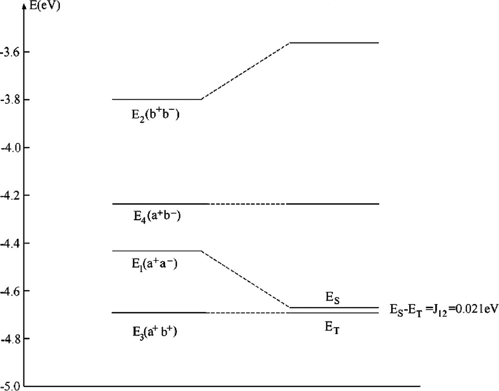
Correlation diagram between the energies of single determinants from DFT and the resulting multiplets of relevance for the magnetic exchange coupling in a [Cu(NH₃)₂(OH)]₂²⁺ model cluster with a ferromagnetic spin alignment.

It is remarkable that ferromagnetic contributions to J₁₂ seem to be realistically described by the LFDFT procedure and our results show that such terms could be indeed rather important (as large as 0.061 eV in the chosen example, see Table 4b). Such terms have been neglected in earlier studies [36] or deemed by physicists to be small [17].

J₁₂(p)^f	J₁₂(p)^af	K₁₂	T₁₂	U
0.121	–0.111	0.061	0.159	0.909

7 Conclusion

The model we present here is simple and easy to implement. The quality of the predictions is exceptional in regard of the low computer time consumption. Keeping in mind that time dependent (TD) DFT is restricted to closed shell molecules an is still problematic for TM complexes and difference dedicated CI approaches [37–39] could be applied with success but only to systems of a smaller size, the model presented here is probably unique to address excited states of molecules with open d- and f-shells. Moreover, the concepts used here (LF theory, Racah parameter) are familiar to all chemists and spectroscopists. Thus, the quantities involved in the calculations provide immediate insights and facilitates communication between theorists and experimentalists. On the basis of our results we can conclude that DFT provides a rigorous interpretation of the LF-parameters and leads to a justification of the parametric structure of the classical LF theory. It is remarkable to mention that a theory which was discovered three quarter of a century ago is still modern.

Acknowledgements

This work was supported by the Swiss National Science Foundation.

Bibliographie

[1] G. Te Velde; F.M. Bickelhaupt; E.J. Baerends; C. Fonesca Guerra; S.J.A. Van Gisbergen; J.G. Snijders; T. Ziegler J. Comput. Chem., 22 (2001), p. 931 (and cited references)

[2] T. Ziegler Chem. Rev., 91 (1991), p. 651

[3] C. Daul Int. J. Quant. Chem., 52 (1994), p. 867

[4] M. Atanasov; C.A. Daul; C. Rauzy; M. Atanasov; C.A. Daul; C. Rauzy Struct. Bond., 367 (2003), p. 737

[5] M. Atanasov; C.A. Daul; C. Rauzy Int. J. Quant. Chem., 102 (2005), p. 119

[6] A. Borel; C.A. Daul; L. Helm Chem. Phys. Lett., 383 (2004), p. 584

[7] M. Atanasov; E.J. Baerends; P. Bättig; R. Bruyndonckx; C. Daul; C. Rauzy; M. Zbiri Chem. Phys. Lett., 399 (2004), p. 433

[8] (a) M. Atanasov, C.A. Daul, Chem. Phys. Lett. 379 (2003) 209 ; (b) M. Atanasov, C.A. Daul, Chem. Phys. Lett. 381 (2003) 584.

[9] P.O. Löwdin Perturbation Theory and Its Applications in Quantum Mechanics (C.H. Wilcox, ed.), Wiley, 1966, pp. 255-294

[10] P.H. Durand; J.P. Malrieu Adv. Chem. Phys., 67 (1987), p. 321

[11] J. des Cloizeaux Nucl. Phys., 20 (1960), p. 321

[12] C.J. Ballhausen; J.P. Dahl Theor. Chim. Acta (Berl.), 34 (1974), p. 169

[13] T. Schönherr, M. Atanasov, H. Adamsky, Comprehensive Coordination Chemsitry II, Vol. 2, Elsevier, 2003, pp. 443–455. And cited original papers of C.K. Jorgensen, C.E. Schäfer, H.-H. Schmidtke.

[14] H. Adamsky; T. Schönherr; M. Atanasov Comprehensive Coordination Chemistry II, Vol. 2, Elsevier, 2003, pp. 661-664

[15] M. Gerloch; J.H. Harding; R. Guy Woolley; M. Atanasov; H.-H. Schmidtke Chem. Phys., 46 (1981), p. 1

[16] E. Van Lenthe; E.J. Baerends; J.G. Snijders J. Chem. Phys., 99 (1993), p. 4597

[17] P.W. Anderson Phys. Rev., 115 (1959), p. 2

[18] P.J. Hay; J.C. Thibeault; R. Hoffmann J. Am. Chem. Soc., 97 (1975), p. 4884

[19] J. Zaanen; G.A. Sawatzky Can. J. Phys., 65 (1987), p. 1262

[20] J. Zaanen; G.A. Sawatzky; J.W. Allen Phys. Rev. Lett., 55 (1985), p. 418

[21] F. Tuczek; E.I. Solomon Coord. Chem. Rev., 219–221 (2001), p. 1075

[22] ADFUserguide (program release 2003.01), http://www.scm.com.

[23] E.J. Baerends; D.E. Ellis; P. Ros Chem. Phys., 2 (1973), p. 42

[24] P.M. Boerrigter; G. te Velde; E.J. Baerends Int. J. Quant. Chem., 33 (1988), p. 87

[25] G. teVelde; E.J. Baerends Comput. Phys., 99 (1992), p. 84

[26] S.H. Vosko; L. Wilk; M. Nusair Cana. J. Phys., 58 (1980), p. 1200

[27] K. Bellafrouh; C.A. Daul; H.U. Güdel; F. Gilardoni; J. Weber Theor. Chim. Acta, 91 (1995), p. 215

[28] L.E. Orgel J. Chem. Soc. (1961), p. 3683

[29] A. Ceulemans; M. Dendooven; L.G. Vanuickenborne Inorg. Chem., 24 (1985), p. 1153 (ibid. 1159)

[30] C. Ribbing; K. Pierloot; A. Ceulemans Inorg. Chem., 37 (1998), p. 5227

[31] M. Atanasov; T. Schönherr; H.-H. Schmidtke Theor. Chim. Acta (Berl), 71 (1987), p. 59

[32] M. Atanasov; T. Schönherr Inorg. Chem., 29 (1990), p. 4545 (and cited ESR and ODMR references)

[33] M. Atanasov; S. Angelov Chem. Phys., 150 (1991), p. 383 (and cited original papers on the Goodenough–Kanamori rules)

[34] D.J. Hodgson Progr. Inorg. Chem., 19 (1975), p. 173

[35] L. Noodleman J. Chem. Phys., 74 (1981), p. 5737

[36] R. Schenker; H. Weihe; H.U. Güdel Inorg. Chem., 38 (1999), p. 5593

[37] J. Miralles; J.-P. Daudey; R. Caballol; J.-P. Malrieu Chem. Phys. Lett., 198 (1992), p. 555

[38] J. Miralles; O. Castell; R. Caballol; J.-P. Malrieu Chem. Phys., 172 (1993), p. 33

[39] F. Neese J. Chem. Phys., 119 (2003), p. 9428

Commentaires - Politique

Ces articles pourraient vous intéresser

Introduction to the intuitive engineering of homogeneous and isotropic two-photon absorbent molecular materials

Rémy Fortrie; Henry Chermette

C. R. Chim (2005)

Les fluorures inorganiques, des matériaux modèles pour tester les méthodes de calcul de paramètres RMN (déplacement chimique et paramètres quadripolaires)

Gilles Silly; Monique Body; Jean-Yves Buzaré; ...

C. R. Chim (2004)

Measurement of short NMR relaxation times: Effect of radio-frequency pulse length

Benjamin Nicot; Marc Fleury; Jacques Leblond

C. R. Chim (2008)