Measurement of short NMR relaxation times: Effect of radio-frequency pulse length

Benjamin Nicot; Marc Fleury; Jacques Leblond

doi:10.1016/j.crci.2007.11.004

Measurement of short NMR relaxation times: Effect of radio-frequency pulse length

Benjamin Nicot ^1,² ; Marc Fleury ¹ ; Jacques Leblond ²

¹ IFP, Département Pétrophysique, 1, avenue de-Bois-Préau, 92852 Rueil-Malmaison cedex, France
² ESPCI, Laboratoire de Physique Thermique, Paris, France

Comptes Rendus. Chimie, GERM 2007, Volume 11 (2008) no. 4-5, pp. 506-514.

Résumé

In certain situations, such as in viscous liquids or nano-porous media, the transversal relaxation time T₂ may become so short that the pulse duration or the detector dead time is no longer negligible. These cases raise fundamental questions about relaxation during the radio-frequency pulses used in classical CPMG or Inversion-Recovery sequences. For an ideal system having a single relaxation time, we examine the effect of the finite pulse duration on the magnetization decay after the pulses occurring in FID, CPMG and Inversion-Recovery sequences. We solved analytically the Bloch equations during and after the pulses and compared the theoretical predictions with experimental data. Finally, we propose approximate simple expressions to correct the sequences for the magnetization attenuation during the pulses. IR curves are affected by transversal relaxation during the pulses, yielding asymmetric curves even if T₁ is very large. The magnetization decay obtained during a CPMG sequence is not affected by relaxation during the pulses. This is valid provided the time origin is chosen in the middle of the first pulse.

Métadonnées

Reçu le : 2007-05-07
Accepté le : 2007-11-06
Publié le : 2007-12-27

DOI : 10.1016/j.crci.2007.11.004

Mots-clés : NMR, Relaxation, CPMG, Inversion-Recovery

Affiliations des auteurs :

Benjamin Nicot ^{1, 2} ; Marc Fleury ¹ ; Jacques Leblond ²

¹ IFP, Département Pétrophysique, 1, avenue de-Bois-Préau, 92852 Rueil-Malmaison cedex, France
² ESPCI, Laboratoire de Physique Thermique, Paris, France

@article{CRCHIM_2008__11_4-5_506_0,
     author = {Benjamin Nicot and Marc Fleury and Jacques Leblond},
     title = {Measurement of short {NMR} relaxation times: {Effect} of radio-frequency pulse length},
     journal = {Comptes Rendus. Chimie},
     pages = {506--514},
     publisher = {Elsevier},
     volume = {11},
     number = {4-5},
     year = {2008},
     doi = {10.1016/j.crci.2007.11.004},
     language = {en},
}

TY  - JOUR
AU  - Benjamin Nicot
AU  - Marc Fleury
AU  - Jacques Leblond
TI  - Measurement of short NMR relaxation times: Effect of radio-frequency pulse length
JO  - Comptes Rendus. Chimie
PY  - 2008
SP  - 506
EP  - 514
VL  - 11
IS  - 4-5
PB  - Elsevier
DO  - 10.1016/j.crci.2007.11.004
LA  - en
ID  - CRCHIM_2008__11_4-5_506_0
ER  -

%0 Journal Article
%A Benjamin Nicot
%A Marc Fleury
%A Jacques Leblond
%T Measurement of short NMR relaxation times: Effect of radio-frequency pulse length
%J Comptes Rendus. Chimie
%D 2008
%P 506-514
%V 11
%N 4-5
%I Elsevier
%R 10.1016/j.crci.2007.11.004
%G en
%F CRCHIM_2008__11_4-5_506_0

Benjamin Nicot; Marc Fleury; Jacques Leblond. Measurement of short NMR relaxation times: Effect of radio-frequency pulse length. Comptes Rendus. Chimie, GERM 2007, Volume 11 (2008) no. 4-5, pp. 506-514. doi : 10.1016/j.crci.2007.11.004. https://comptes-rendus.academie-sciences.fr/chimie/articles/10.1016/j.crci.2007.11.004/

Version originale du texte intégral

Le texte intégral ci-dessous peut contenir quelques erreurs de conversion par rapport à la version officielle de l'article publié.

1 Introduction

NMR relaxation time measurements on liquids performed at moderate or low field provide useful information about molecular dynamics. For example, viscosity can be deduced from transversal relaxation time over a very wide range of values spanning several decades. In porous media, a pore size information can be obtained from transversal and longitudinal relaxation times. In most situations, the transversal and longitudinal relaxation times are much larger than the radio-frequency (r.f.) pulse durations τ_p and the dead time of the detector τ_d. In these cases, the Carr–Purcell–Meiboom–Gill (CPMG) [1,2] and the Inversion-Recovery (IR) [3] sequences are perfectly adapted to determine T₂, T₁ and the total magnetization, without correction for quantitative analysis. In contrast, in very viscous liquids where T₁ ≫ T₂, the transversal relaxation time can become so short that the conditions T₂ ≫ τ_p or T₂ ≫ τ_d may not be satisfied. We focus in this paper on these cases and we consider the evolution of the magnetization during the pulses.

The effect of finite pulse duration and relaxation during the pulses has been of concern very early in the development of NMR. In particular in the study of chemical exchange [4,5], the relaxation during pulses has important consequences and can be used to select different protons in high-resolution NMR [6]. In this work, we consider low-resolution experiments designed to provide quantitative information about proton species relaxing at different rates to identify their contribution in the system studied. For example, in liquids, we expect to obtain the contribution of high molecular weight components relative to low molecular weight, and for a confined liquid in a porous media, we expect to obtain a precise partitioning of the pore space.

We will first recall the Bloch equations and show that they can be used for the calculation of the magnetization decay during the pulses. Then we present the analytical method to solve the Bloch equations during the pulses as well as the experimental method to observe the effect of pulse duration. The results of the calculation for individual pulses are presented next, along with an experimental validation performed on a FID sequence. Finally we show theoretically and experimentally the effects of relaxation during the pulses on CPMG and IR measurements and propose simple analytical formulae to perform corrections when necessary.

2 Background: Bloch equations and underlying assumptions

Let us consider one set of spins, characterized by:

• a given dipolar interaction correlation time τ_c,
• a given mean square of the dipolar interaction tensor components,

and consequently, by:

• a longitudinal relaxation time T₁;
• a transversal relaxation time T₂.

We will note:

• Oxyz the laboratory frame of reference with Oz along the magnetic induction, B₀;
• OXYz the frame of reference rotating around Oz at the angular frequency ω ≈ ω₀ = −γB₀, where γ is the gyromagnetic factor.

During each sequence the evolution of the magnetization of this spin package is well described by the Bloch equations [7] under the following conditions:

• a homogeneous static magnetic induction, B₀;
• B₁ ≪ B₀, where B₁ is the amplitude of the magnetic induction $\vec{B_{1}}$ perpendicular to $\vec{B_{0}}$ , and rotating at the angular frequency ω;
• <ω²>^1/2τ_c < 1 where <ω²> is the second moment of the local dipolar interaction. According to the Bloembergen, Purcell and Pound (BPP) theory [8], this condition is fulfilled if T₂ > T_2limit ≈ 11 μs for an inter-proton distance b = 1.78 Å, which corresponds to the distance between two hydrogen atoms in the methane molecule.

Under these conditions, the effective static induction in the rotating frame OXYz is:

\vec{B_{eff}} = (B_{0} + \frac{ω}{γ}) \vec{k} + \vec{B_{1}} = \frac{Δ ω \vec{k} - \vec{ω_{1}}}{γ}

(1)

where

\vec{ω_{1}} = - γ \vec{B_{1}}

, Δω = ω − ω₀ and

\vec{i}, \vec{j}, \vec{k}

are the unit vectors of the rotating frame. In this rotating frame, the Bloch equations become:

\frac{ⅆ \vec{M}}{ⅆ t} = γ (\vec{M} \land \vec{B_{eff}}) - \frac{M_{X} \vec{i} + M_{Y} \vec{j}}{T_{2}} - \frac{M_{z} - M_{0}}{T_{1}} \vec{k}

(2)

where M_X, M_Y, M_z are the components of the magnetization

\vec{M}

in that frame, and M₀, the magnetization at thermal equilibrium along Oz. The use of the Bloch equations during the r.f. pulses is suitable as far as 1/T_2ρ = 1/2(1/T₁ + 1/T₂) and 1/T_1ρ = 1/T₂, i.e. when ω₁τ_c ≪ 1, where T_1ρ and T_2ρ are the relaxation times in the rotating frame in the presence of B₁.

3 Analytical and experimental methods

3.1 Resolution of the Bloch equations during a r.f. pulse

Bloch equations were solved during the three different pulses occurring in the CPMG and IR sequences. In each case, the magnetization state before the application of the pulses is linked to the sequences as follows:

• application of a π/2)_X pulse when the magnetization is initially along the z axis. This case corresponds to the 90° pulses applied in CPMG, IR and Free Induction Decay (FID) measurements;
• application of a π)_X pulse when the magnetization is initially along z. This case corresponds to the inversion pulse in the IR measurement;
• application of a π)_Y pulse when the initial magnetization is mainly along Y. This case corresponds to a 180° refocusing pulse in the CPMG sequence.

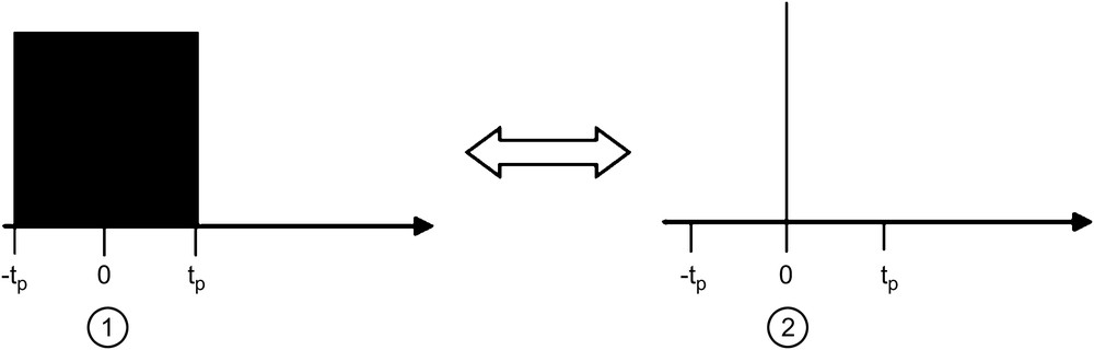
The analytical resolution was performed for a square pulse (pulse 1 in Fig. 1) and for an “ideal” pulse of zero duration occurring at time t = 0 and producing a perfect tilt of the magnetization (pulse 2 in Fig. 1). The analytical calculations, detailed in the Appendix, were performed up to the order ɛ², where $ɛ^{2} = 1 / 2 ω_{1} T_{2}$ , neglecting the effect of the longitudinal relaxation (T₁ ≫ 2t_p).

Fig. 1
Real r.f. pulse (1) and ideal r.f. pulse (2).

3.2 Experiments

All the experiments have been carried out on a Maran Ultra 23-MHz proton spectrometer from Oxford Instruments. The characteristic time of the free induction decay due to magnetic field inhomogeneities $T_{2}^{*}$ is about 1.5 ms. At a constant r.f. amplitude we will note, respectively, τ_p and 2τ_p the π/2 and π pulse durations. Pulse durations were accurately determined using the standard train90 and train180 pulse sequences. The minimum π/2 pulse duration is τ_p _min = 6 μs. The dead time (probe + filter) is τ_d = 12 μs.

In order to compare experiments and calculations, we checked that the conditions for applying the Bloch equations are valid:

• the condition $T_{2} ≪ T_{2}^{*}$ is fulfilled and the B₀ induction can be considered homogeneous,
• the condition B₁ ≪ B₀ because the minimum π/2 pulse duration is τ_p _min = 6 μs, corresponding to ∼42 kHz,
• the relaxation is exponential and not Gaussian.

Viscous hydrocarbon fluids are our main interest, but they usually exhibit a broad distribution of relaxation times [9] and are not suitable for the present study. For the FID and IR tests, we used instead a sample of glycerol at a temperature of −10 °C. At that temperature, we measured T₁ and T₂ values, respectively, of 0.46 ms and 44 ms. For the CPMG tests, we also used glycerol but a temperature of 30 °C (T₂ = 25 ms, T₁ = 43 ms) and we varied the inter-echo time TE = 2τ from 100 up to 600 μs. Hence, the ratio TE/2τ_p varies from 8.3 to 50. In addition, we decreased the number of echoes N_ech in order to maintain the ratio τ/N_ech constant, i.e. the magnetization decay is recorded over a fixed time interval. In all cases, the zero time origin is at the middle of the first pulse.

4 Results for individual pulses

We present here the results of the calculation for the three pulses used in the IR and CPMG sequences. We note t_p the end of the r.f. pulse with a time origin located at the centre of the pulse, τ_p the duration of a π/2 pulse (hence t_p = τ_p/2 for a π/2 pulse and t_p = τ_p for a π pulse), and M_X₀, M_Y₀, M_z₀, the components of $\vec{M}$ in the rotating frame at time t = −t_p. From the values of the magnetization components after the three different pulses (Table 1) under study, we see that there is no difference between the real and ideal pulses for three cases out of nine (Table 1). However, this is true only if one chooses the time origin at the centre of the pulse. For these cases, the considered magnetization component is along the rotation axis. Otherwise, the differences occurring between real and ideal pulses reveal the effect of T₂ relaxation during the pulses. For example, starting from M_X₀ = 0, M_Y₀ = 0 and M_z₀ = M₀ (FID sequence), a residual M_z component remains after the application of a π/2)_X pulse (Fig. 2):

M_{z} (t_{p}) = M_{0} \frac{π ɛ^{2}}{4} \exp (- \frac{τ_{p}}{2 T_{2}})

(3)

Starting from M_X₀ = M_Y₀ = 0 and M_z₀ = M₀, the effect of relaxation during a π/2)_X pulse (duration τ_p) can be obtained from Table 1:

\begin{array}{l} M_{X} (t_{p}) = 0 \\ M_{Y} (t_{p}) = M_{0} \exp (- \frac{τ_{p}}{2 T_{2}}) \\ M_{z} (t_{p}) \approx M_{0} \frac{π ɛ^{2}}{4} \exp (- \frac{τ_{p}}{2 T_{2}}) \end{array}

(4)

As already mentioned, the magnetization is not perfectly tilted along OY and the effective tilt angle is less than 90°. Considering the measurable component M_Y, there is an attenuation due to the decrease of the overall magnetization modulus, and to the imperfect tilt angle. We define the attenuation Att_π/2 of the M_Y component after a π/2)_X pulse as:

{Att}_{π / 2} (t_{p}) = \frac{M_{Y} (t_{p})}{M_{0}} \approx \exp (- \frac{τ_{p}}{2 T_{2}})

(5)

Starting from M_X₀ = M_Y₀ = 0 and M_z₀ = M₀, the effect of relaxation during a π)_X pulse (pulse duration 2τ_p) can be obtained from Table 1:

\begin{array}{l} M_{X} (t_{p}) = 0 \\ M_{Y} (t_{p}) \approx M_{0} \frac{π ɛ^{2}}{2} \exp (- \frac{τ_{p}}{T_{2}}) \\ M_{z} (t_{p}) = - M_{0} \exp (- \frac{τ_{p}}{T_{2}}) \end{array}

(6)

In this case, the effective tilt angle is 180°, the remaining magnetization along Y is negligible, and there is an attenuation of the magnetization amplitude. Similarly, we define the attenuation of the M_z component after a π)_X pulse as:

{Att}_{π} (t_{p}) = \frac{M_{z} (t_{p})}{- M_{0}} \approx \exp (- \frac{τ_{p}}{T_{2}})

(7)

Finally, whatever the magnetization components M_X₀, M_Y₀ and M_z₀ may be, the effect of relaxation during a π)_Y pulse (pulse duration 2τ_p) can be obtained from Table 1:

M_{Y} (t_{p}) = M_{Y 0} \exp (- \frac{2 τ_{p}}{T_{2}})

(8)

It is obvious that when rotating around the Y axis during the pulse, the M_Y component relaxes exponentially with a time constant T₂.

R.f. pulse	M_X (t_p)	M_Y (t_p)	M_z (t_p)
π/2)_X	1	$M_{X 0} ⅇ^{- \frac{τ_{p}}{T_{2}}}$	$(M_{z 0} + \frac{π ɛ^{2}}{4} M_{Y 0}) ⅇ^{- \frac{τ_{p}}{2 T_{2}}}$	$(- M_{Y 0} + \frac{π ɛ^{2}}{4} M_{z 0}) ⅇ^{- \frac{τ_{p}}{2 T_{2}}}$
2	$M_{X 0} ⅇ^{- \frac{τ_{p}}{T_{2}}}$	$M_{z 0} ⅇ^{- \frac{τ_{p}}{2 T_{2}}}$	$M_{Y 0} ⅇ^{- \frac{τ_{p}}{2 T_{2}}}$

π)_X	1	$M_{X 0} ⅇ^{- \frac{2 τ_{p}}{T_{2}}}$	$(- M_{Y 0} + \frac{π ɛ^{2}}{2} M_{z 0}) ⅇ^{- \frac{τ_{p}}{T_{2}}}$	$(- M_{z 0} - \frac{π ɛ^{2}}{2} M_{Y 0}) ⅇ^{- \frac{τ_{p}}{T_{2}}}$
2	$M_{X 0} ⅇ^{- \frac{2 τ_{p}}{T_{2}}}$	$- M_{Y 0} ⅇ^{- \frac{τ_{p}}{T_{2}}}$	$- M_{z 0} ⅇ^{- \frac{τ_{p}}{T_{2}}}$

π)_Y	1	$(- M_{X 0} - \frac{π ɛ^{2}}{2} M_{z 0}) ⅇ^{- \frac{τ_{p}}{T_{2}}}$	$M_{Y 0} ⅇ^{- \frac{2 τ_{p}}{T_{2}}}$	$(- M_{z 0} + \frac{π ɛ^{2}}{2} M_{X 0}) ⅇ^{- \frac{τ_{p}}{T_{2}}}$
2	$- M_{X 0} ⅇ^{- \frac{τ_{p}}{T_{2}}}$	$M_{Y 0} ⅇ^{- \frac{2 τ_{p}}{T_{2}}}$	$- M_{z 0} ⅇ^{- \frac{τ_{p}}{T_{2}}}$

Fig. 2
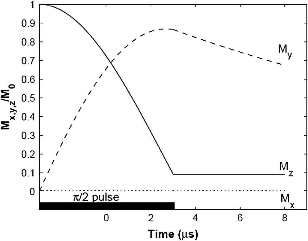
Calculation of M_X, M_Y, and M_z as a function of time during and after a π/2)_X pulse for τ_p = 6 μs, T₁ = 10 s and T₂ = 20 μs.

In practical situation, the detection of the magnetization is only possible after a dead time τ_d which is typically of the order of 10 μs. The resulting attenuation is then expressed as:

{Att}_{dead} = \exp (- \frac{τ_{d}}{T_{2}})

(9)

and the magnetization is then given by (in the case of a π/2 pulse):

M_{Y} (t_{p} + τ_{d}) \approx M_{0} {Att}_{π / 2} (t_{p}) {Att}_{dead}

(10)

To test experimentally Eq. (10), we used glycerol relaxing at T₂ = 460 μs at −10 °C and we varied the π/2 pulse duration τ_p from 6.2 μs up to 380 μs. Therefore, the τ_p/T₂ ratio varies from 0.01 to 0.83. There is a good agreement between experimental data (first FID points) and the total predicted attenuation Att_π/2Att_dead (Fig. 3). Note that this curve does not reach 1 for small values of τ_p/T₂. Indeed, we varied the pulse duration τ_p and not the T₂ value, so that there is a constant attenuation factor Att_dead, corresponding to:

{Att}_{dead} = \exp (- \frac{τ_{d}}{T_{2}}) = \exp (- \frac{12}{460}) \approx 0.97

(11)

Fig. 3
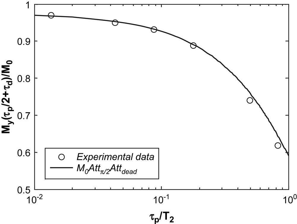
Amplitude of the first measurable point of the FID versus τ_p/T₂ for a glycerol sample at −10 °C; the spectrometer dead time τ_d = 12 μs is taken into account in the analytic formula, see Eq. (10).

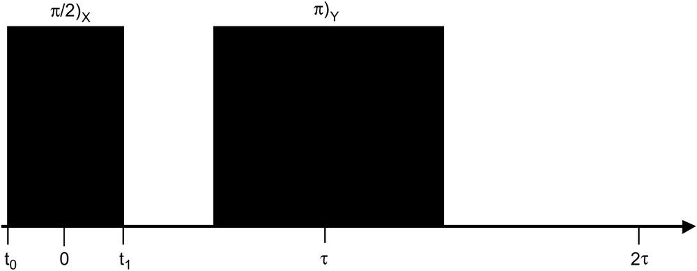
5 Results for the IR sequence

We treat here the Inversion-Recovery (IR) pulse sequence commonly used for T₁ measurements and described in Fig. 4. We can calculate the magnetization components during this sequence using the results obtained for individual pulses (Table 1).

Fig. 4
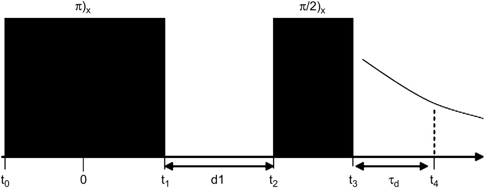
Inversion-Recovery pulse sequence.

At t₀ = −τ_p, the magnetization is along z, therefore:

\begin{array}{l} M_{X} (t_{0}) = 0 \\ M_{Y} (t_{0}) = 0 \\ M_{z} (t_{0}) = M_{0} \end{array}

(12)

After the π)_X pulse, at t₁ = τ_p the magnetization components are:

\begin{array}{l} M_{X} (t_{1}) = 0 \\ M_{Y} (t_{1}) \approx M_{0} \frac{π ɛ^{2}}{2} \exp (- \frac{τ_{p}}{T_{2}}) \\ M_{z} (t_{1}) = - M_{0} \exp (- \frac{τ_{p}}{T_{2}}) \end{array}

(13)

Then, the magnetization components relax exponentially, M_X and M_Y decreasing with a time constant T₂ and M_z with a time constant T₁, during the time d₁. So, at time t₂ = τ_p + d₁ the magnetization components can be written as:

\begin{array}{l} M_{X} (t_{2}) = 0 \\ M_{Y} (t_{2}) \approx M_{0} \frac{π ɛ^{2}}{2} \exp (- \frac{τ_{p}}{T_{2}}) \exp (- \frac{d_{1}}{T_{2}}) \\ M_{z} (t_{2}) = M_{0} + (- M_{0} \exp (- \frac{τ_{p}}{T_{2}}) - M_{0}) \exp (- \frac{d_{1}}{T_{1}}) \end{array}

(14)

After the π/2)_x pulse, at time t₃ = τ_p + d₁ + τ_p, the magnetization components are:

\begin{array}{l} M_{X} (t_{3}) = 0 \\ M_{Y} (t_{3}) \approx [M_{0} - (M_{0} \exp (- \frac{τ_{p}}{T_{2}}) + M_{0}) \exp (- \frac{d_{1}}{T_{1}}) + M_{0} \frac{π ɛ^{2}}{4} \frac{π ɛ^{2}}{2} \exp (- \frac{τ_{p}}{T_{2}}) \exp (- \frac{d_{1}}{T_{2}})] \exp (- \frac{τ_{p}}{2 T_{2}}) \\ M_{z} (t_{3}) \approx [\frac{π ɛ^{2}}{2} M_{0} \exp (- \frac{τ_{p}}{T_{2}}) \exp (- \frac{d_{1}}{T_{2}}) + \frac{π ɛ^{2}}{2} (M_{0} + (M_{0} \exp (- \frac{τ_{p}}{T_{2}}) - M_{0}) \exp (- \frac{d_{1}}{T_{1}}))] \exp (- \frac{τ_{p}}{2 T_{2}}) \end{array}

(15)

After a dead time τ_d, neglecting terms of order ɛ⁴ in Eq. (15), the detected M_Y component at time t₄ = τ_p + d₁ + τ_p + τ_d can be written as:

M_{Y} (t_{4}) = [M_{0} - (M_{0} \exp (- \frac{τ_{p}}{T_{2}}) + M_{0}) \exp (- \frac{d_{1}}{T_{1}})] \exp (- \frac{τ_{p}}{2 T_{2}}) \exp (- \frac{τ_{d}}{T_{2}})

(16)

As a consequence, even if the T₁ measurement is affected by transversal relaxation during the pulses, the M_Y component relaxes exponentially when d₁ is varied. A typical Inversion-Recovery curve is shown in Fig. 5. Using Eq. (16), we can write the expressions of M_Y (t₄, d₁ → 0) and M_Y (t₄, d₁ → ∞) as follows:

M_{Y} (t_{4}, d_{1} \to 0) = - M_{0} \exp (- \frac{τ_{p}}{T_{2}}) \exp (- \frac{τ_{p}}{2 T_{2}}) \exp (- \frac{τ_{d}}{T_{2}})

(17)

M_{Y} (t_{4}, d_{1} \to ∞) = M_{0} \exp (- \frac{τ_{p}}{2 T_{2}}) \exp (- \frac{τ_{d}}{T_{2}})

(18)

Fig. 5
Typical Inversion-Recovery curve.

Thus, using the expressions of the attenuations defined in Eqs. (5), (7) and (9), one can write these expressions as:

M_{Y} (t_{4}, d_{1} \to 0) = - M_{0} {Att}_{π} (τ_{p}) {Att}_{π / 2} (τ_{p} / 2) {Att}_{dead}

(19)

M_{Y} (t_{4}, d_{1} \to ∞) = M_{0} {Att}_{π / 2} (τ_{p} / 2) {Att}_{dead}

(20)

The common way to treat the IR curves is to apply the following transform:

T (d_{1}) = M_{Y} (d_{1} \to ∞) (1 - \frac{M_{Y} (d_{1})}{M_{Y} (d_{1} \to ∞)})

(21)

yielding a curve decreasing from M_Y(d₁ → ∞) − M_Y(d₁ → 0) to zero. This curve is then treated as an exponential decay. In consequence, the magnetization amplitude of a T₁ component can be defined as M_Y(d₁ → ∞) − M_Y(d₁ → 0), rather than the classically expected amplitude 2M₀ obtained when T₂ ≫ τ_p and τ_d. The amplitude ratio Att_IR is:

{Att}_{IR} = \frac{M_{Y} (d_{1} \to ∞) - M_{Y} (d_{1} \to 0)}{2 M_{0}}

(22)

Using Eqs. (19) and (20), one can write this amplitude ratio as:

{Att}_{IR} = \frac{[1 + {Att}_{π} (τ_{p})] {Att}_{π / 2} (τ_{p} / 2) {Att}_{dead}}{2}

(23)

The full IR sequence has been calculated for different values of τ_p (Fig. 6). The dead time has been set to zero for simplicity.

Fig. 6
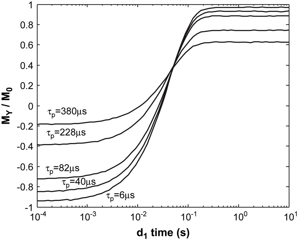
Calculated Inversion-Recovery curves for different pulse durations with τ_d = 0, T₁ = 1 ms and T₂ = 20 μs.

As a result of Eqs. (19) and (20), M_Y(d₁ → 0) is more attenuated than M_Y(d₁ → ∞), yielding non-symmetric curves, as presented in Fig. 6. However, despite this asymmetry, the relaxation time T₁ is constant, as predicted by Eq. (16).

In order to obtain an experimental verification of Eq. (23), T₁ measurements were performed for different pulse durations τ_p on a glycerol sample at −10 °C (T₂ = 460 μs). The detected amplitude [M_Y (d_1max) − M_Y(d_1min)]/2M₀ with d_1max = 10 s and d_1min = 10 μs as a function of τ_p/T₂ is in agreement (Fig. 7) with the analytical attenuation Att_IR given by Eq. (23). For each IR measurement (Fig. 8), non-symmetric curves are measured, as predicted, but the same T₁ value (46 ms) is deduced independently of the pulse duration.

Fig. 7
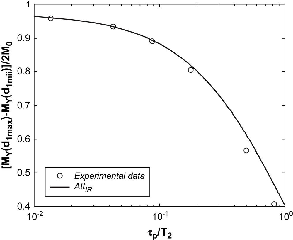
Total amplitude from IR measurements versus τ_p/T₂, glycerol sample at −10 °C; a dead time τ_d of 12 μs is taken into account in the analytic formula given in Eq. (23).

Fig. 8
IR measurements for a glycerol sample at −10 °C for different values of pulse duration at resonance condition; the same relaxation time is obtained for all curves (T₁ = 46 ms).

6 Results for the CPMG sequence

We have already studied separately the effect of the pulses used in a CPMG measurement (Table 1). If we consider the pulse sequence described in Fig. 9, we can calculate the magnetization components during the sequence. At t₀ = −τ_p/2, the magnetization is along Oz, therefore:

\begin{array}{l} M_{X} (t_{0}) = 0 \\ M_{Y} (t_{0}) = 0 \\ M_{z} (t_{0}) = M_{0} \end{array}

(24)

Fig. 9
CPMG pulse sequence considered in this work.

After the π/2)_X pulse, at t₁ = τ_p/2, the magnetization components are:

\begin{array}{l} M_{X} (t_{1}) = 0 \\ M_{Y} (t_{1}) = M_{0} \exp (- \frac{τ_{p}}{2 T_{2}}) \\ M_{z} (t_{1}) \approx M_{0} \frac{π ɛ^{2}}{4} \exp (- \frac{τ_{p}}{2 T_{2}}) \end{array}

(25)

Then the M_Y component relaxes exponentially without any effect of the π)_Y pulses during a time 2τ − t. So at t = 2τ, the M_Y component can be written as:

M_{Y} (2 τ) = M_{0} \exp (- \frac{τ_{p}}{2 T_{2}}) \exp (- \frac{2 τ - t_{1}}{T_{2}}) = M_{0} \exp (- \frac{2 τ}{T_{2}})

(26)

As a consequence, if the time origin is taken at the middle of the first pulse, relaxation during the pulses does not affect the results of the CPMG measurement.

We have calculated the full sequence by Bloch equations, resolution for an extreme case, where T₂ (= 40 μs) ≪ T₁ (= 10 s) and τ_p = 20 μs. We simulated three echoes with a half inter-echo time τ = 30 μs (Fig. 10).

Fig. 10
Magnetization (M_X, M_Y, M_z) versus time during a CPMG sequence (3 echoes with τ = 30 ms, π/2 pulse length τ_p = 20 μs, T₁ = 10 s and T₂ = 40 μs).

We also tested the analytical result of Eq. (26) experimentally. Several CPMG measurements were performed on a glycerol sample at 30 °C (T₂ = 44 ms), as described in a previous section. The measured magnetization decays were fitted using a single exponential component and each experiment led to the same T₂ value whatever the τ value or the number of echoes or the total π pulse duration in the CPMG sequence. This is true if the magnetization is recorded as a function of time counted from the middle of the first pulse, in particular for long π pulse. A simple fitting procedure using the data points at time t = 2nτ (n = 1, 2…) yields the total magnetization M₀ and T₂. According to these results, we conclude that the CPMG sequence has theoretically the ability to detect both the amplitude and time constant for very short T₂ values. However, when a distribution of relaxation time is present in the fluid (as often encountered), the shortest components are described only by a few echoes. Therefore, in a multi-exponential fitting, the weight of the longest components is much larger, yielding a poor determination of the short components.

7 Conclusion

The calculations presented in this article treat the problem of short T₂ relaxation time detection. The transversal relaxation during the pulses has been calculated by analytical resolution of Bloch equations. The remarkable agreement observed between experimental and theoretical attenuations establishes the adequacy of these equations to solve the specific problem of relaxation during the pulses. Although the description of the attenuation using simple exponential functions is not exact, it is sufficient to represent experimental results.

The main conclusions concerning relaxation time measurements are as follows:

• for the FID sequence, relaxation during the pulse yields underestimated magnetization values. This magnetization loss is predicted by Eq. (10), in good agreement with experimental data;
• for the CPMG sequence, we have shown that there is no effect of relaxation during the pulses. Neither the number nor the duration of the pulses will affect the determination of the relaxation time T₂;
• for the IR sequence, transversal relaxation during pulses and dead time yields a non-negligible underestimation of magnetization and asymmetric IR curves. This magnetization loss is predicted by Eq. (23), in good agreement with experimental data. However, the T₁ value deduced from IR curves is not affected by the asymmetry.

Appendix Analytical resolution of the Bloch equations during a r.f. pulse

We analyse the effect of a r.f. pulse during a time interval [−t_p; t_p], neglecting the effect of the longitudinal relaxation (T₂ ≪ T₁). We note $\vec{ω_{1}} = - γ \vec{B_{1}}$ , τ_p, the π/2 r.f. pulse duration, and M_X₀, M_Y₀, M_z₀, the components of $\vec{M}$ in the rotating frame at time t = −t_p. Let us consider two typical cases.

• Case 1: when $\vec{B_{1}}$ is applied along OX in the rotating frame. Bloch equations become:

\frac{ⅆ M_{X}}{ⅆ t} = - \frac{M_{X}}{T_{2}}; \frac{ⅆ M_{Y}}{ⅆ t} = - \frac{M_{Y}}{T_{2}} - ω_{1} M_{z}; \frac{ⅆ M_{z}}{ⅆ t} = ω_{1} M_{Y}

(A1)

If

ɛ^{2} = 1 / 2 ω_{1} T_{2} \leq 1

, for

- t_{p} < t < t_{p}

, the solution is:

\begin{array}{l} M_{X} (t) = M_{X 0} \exp (- \frac{t + t_{p}}{T_{2}}) \\ M_{Y} (t) = \exp (- \frac{t + t_{p}}{2 T_{2}}) (M_{Y 0} \cos q (t + t_{p}) + M_{z 0} \sin q (t + t_{p})) \\ M_{z} (t) = \exp (- \frac{t + t_{p}}{2 T_{2}}) (M_{z 0} \cos q (t + t_{p}) - M_{Y 0} \sin q (t + t_{p})) \end{array}

(A2)

with

q = ω_{1} \sqrt{1 - ɛ^{2}}

.

• Case 2: when $\vec{B_{1}}$ is applied along OY in the rotating frame. Bloch equations become:

\frac{ⅆ M_{X}}{ⅆ t} = - \frac{M_{X}}{T_{2}} + ω_{1} M_{z}; \frac{ⅆ M_{Y}}{ⅆ t} = - \frac{M_{Y}}{T_{2}}; \frac{ⅆ M_{z}}{ⅆ t} = - ω_{1} M_{X}

(A3)

If

ɛ^{2} = 1 / 2 ω_{1} T_{2} \leq 1

, for

- t_{p} < t < + t_{p}

, the solution is:

\begin{array}{l} M_{X} (t) = \exp (- \frac{t + t_{p}}{2 T_{2}}) (M_{Y 0} \cos q (t + t_{p}) - M_{z 0} \sin q (t + t_{p})) \\ M_{Y} (t) = M_{X 0} \exp (- \frac{t + t_{p}}{T_{2}}) \\ M_{z} (t) = \exp (- \frac{t + t_{p}}{2 T_{2}}) (M_{z 0} \cos q (t + t_{p}) + M_{Y 0} \sin q (t + t_{p})) \end{array}

(A4)

Next, we will consider the case where ɛ ≪ 1, corresponding to the operating range of the NMR technique, so that we limit the development of sin qt and cos qt up to ɛ² in Eqs. A2 and A4. The components of

\vec{M}

obtained at t_p are defined:

• after a π/2)_X r.f. pulse, corresponding to $t_{p} = τ_{p} / 2$ , by:

\begin{array}{l} M_{X} (t_{p}) = M_{X 0} \exp (- \frac{τ_{p}}{T_{2}}) \\ M_{Y} (t_{p}) = \exp (- \frac{τ_{p}}{2 T_{2}}) (\frac{π ɛ^{2}}{4} M_{Y 0} + M_{z 0}) \\ M_{z} (t_{p}) = \exp (- \frac{τ_{p}}{2 T_{2}}) (\frac{π ɛ^{2}}{4} M_{z 0} - M_{Y 0}) \end{array}

(A5)

• after a π)_X r.f. pulse, corresponding to $t_{p} = τ_{p}$ , by

\begin{array}{l} M_{X} (t_{p}) = M_{X 0} \exp (- \frac{2 τ_{p}}{T_{2}}) \\ M_{Y} (t_{p}) = \exp (- \frac{τ_{p}}{T_{2}}) (- M_{Y 0} + \frac{π ɛ^{2}}{2} M_{z 0}) \\ M_{z} (t_{p}) = \exp (- \frac{τ_{p}}{T_{2}}) (- M_{z 0} - \frac{π ɛ^{2}}{2} M_{Y 0}) \end{array}

(A6)

• after a π)_Y r.f. pulse, corresponding to $t_{p} = τ_{p}$ ,

\begin{array}{l} M_{X} (t_{p}) = \exp (- \frac{τ_{p}}{T_{2}}) (- M_{X 0} - \frac{π ɛ^{2}}{2} M_{z 0}) \\ M_{Y} (t_{p}) = M_{Y 0} \exp (- \frac{2 τ_{p}}{T_{2}}) \\ M_{z} (t_{p}) = \exp (- \frac{τ_{p}}{T_{2}}) (- M_{z 0} + \frac{π ɛ^{2}}{2} M_{X 0}) \end{array}

(A7)

Bibliographie

[1] H. Carr; E. Purcell Phys. Rev., 94 (1954), p. 630

[2] S. Meiboom; D. Gill Rev. Sci. Instrum., 29 (1958), p. 688

[3] R. Vold; J. Waugh; M. Klein; D. Phelps J. Chem. Phys., 48 (1968) no. 8, p. 3831

[4] C.S. Johnson; M. Saunders J. Chem. Phys., 43 (1965), p. 4170

[5] D. Lankhorst; J. Schriever; J.C. Leyte J. Magn. Reson., 51 (1983), p. 430

[6] R. Freeman; S. Wittekoek J. Magn. Reson., 1 (1969), p. 238

[7] F. Bloch Phys. Rev., 70 (1946), p. 460

[8] N. Bloembergen; E. Purcell; R. Pound Phys. Rev., 73 (1948), p. 679

[9] K.J. Dunn; D.J. Bergman; G.A. La Torraca Nuclear Magnetic Resonance, Petrophysical and Logging applications, Seismic Exploration, vol. 32, Pergamon, 2002

Commentaires - Politique