Automatic first-order multiplet analysis in liquid-state NMR

Élise Prost; Stéphane Bourg; Jean-Marc Nuzillard

doi:10.1016/j.crci.2005.05.012

Résumés

Anglais
Français

The extraction of coupling constant values from NMR spectra is an important step in assigning the configuration of organic molecules. A method for the automatic multiplet analysis in weakly coupled spin systems is described here. It relies on a multi-step procedure that forms the AUJ (AUtomatic J) algorithm. Tolerance to low-magnitude second-order effects is achieved by an efficient multiplet centering and symmetrization step. Time-domain signal analysis through a linear model produces a raw evaluation of coupling constants and their associated multiplicities. The final result is obtained through numerical optimization of the multiplet parameters. Two examples are presented, one from an experimental spectrum, and the other one, of higher complexity, from a computer-simulated multiplet. .

L'extraction des valeurs des constantes de couplage présentes dans les spectres de RMN est une étape importante pour l'attribution des configurations dans les molécules organiques. Une méthode d'analyse automatique de s multiplets au premier ordre est décrite ici, fondée sur une procédure multi-étape qui constitue l'algorithme AUJ (AUtomatic J). La tolérance aux faibles effets de second ordre est assurée par une étape efficace de centrage et de symétrisation. L'analyse du signal dans le domaine des temps utilisant un modèle linéaire produit une première évaluation des constantes de couplage et des multiplicités associées. Le résultat final est obtenu par optimisation numérique des paramètres du multiplet. Deux exemples d'application sont présentés : l'un traite d'un multiplet expérimental et l'autre d'un multiplet plus complexe, obtenu par simulation. .

1 Introduction

The spin–spin coupling analysis of 1D NMR spectra describes how nuclei are scalarly coupled within molecules. Scalar couplings are important NMR parameters that provide constraints for the building of 3-D molecular structures [1]. The high magnetic fields at which NMR is performed nowadays reduce the probability of strongly coupled homonuclear spin systems, so that first-order analysis is most often sufficient for measuring coupling constants. Each multiplet can therefore be analyzed independently of the others within the same spin system. The automatic extraction of coupling constants is a problem to which solutions have already been proposed ([2–11], and references cited therein). Human interpretation of a multiplet structure relies on the recognition of elementary peak cluster shapes [12]. Automated methods for first order multiplet analysis mimic this process [11].

A method based on time-domain analysis has already been described by our group [13,14]. Its basic principle was later extended to increase its performance. This communication describes the process that is presently implemented in the AUJ (automatic J couplings) computer software (www.univ-reims.fr/LSD/JmnSoft/Auj).

AUJ is implemented as a GIFA [15] macro command that performs some pre-processing and calls a binary program whose source file is written in C language. The latter uses a library that contains the truely active part of the AUJ algorithm and that is designed to be invoked from any type of NMR processing software. The library uses the time-domain data as input and produces a set of coupling constants as well as the corresponding reconstructed time-domain signal.

2 Process outline

Analysis starts with data point extraction of the user-selected multiplet. The multiplet is then converted to complex time-domain data by inverse Fourier transformation. Alternatively, a column of a 2-D J-resolved spectrum can also be simply extracted by the user and back-converted to real time-domain data. The AUJ algorithm is able to handle both input types. Complex data is supposed to originate from a non-centered non-symmetrical multiplet and therefore must be transformed to real data (step 1). The ‘log-abs’ algorithm [13,14] is then used (step 2) to produce a 1-D J-spectrum that is then optimized (step 3) and analyzed to produce a first set of coupling constants and multiplicities (step 4). At this stage, J values can be accurate but multiplicities are usually not. The latter are optimized (step 5) and the resulting values used to refine the final J values (step 6). Finally, the centered multiplet (when input data is complex), the reconstructed time-domain data, and the J values are exported back to the calling GIFA macro command and made visible through its graphical user interface, so that an algorithm failure is immediately visible. The ratio of the spectral noise level with the root-mean-square deviation between original and reconstructed multiplets is also a good performance indicator. The analysis process depends on empirically adjusted parameters whose default values, provided in the following paragraphs, can easily be adjusted by means of a single control panel. In practice, the proposed defaut parameter values fit well with most of the situations that were tested by the authors.

2.1 Step 1: Multiplet centering and symmetrization

Time-domain data is first zero-filled (16 times by default) to obtain a high resolution multiplet by Fourier transformation. Then, a pivot frequency is searched so that frequency reversal around the pivot point leads to a spectrum that looks, at best, identical to the original one. Reversal and comparison are not directly performed on the high-resolution spectrum but on a binary-valued version of it that is built as follows. The real part of the spectrum is first divided by its Euclidian norm. Each value in the normalized spectrum is replaced by 1 if its value is greater than a given threshold (0.03 by default) and, if not, replaced by 0. The pivot position is selected so that the number of ones is maximum in the point-by-point product of the binary spectrum by its reversed version. The optimum pivot frequency value is used to frequency shift the original time-domain signal by multiplying it by the adequate linear phase ramp function. Frequency symmetrization is achieved de facto by setting the imaginary part of the resulting time-domain data to zero. Centering failure may occur for strongly unsymmetrical multiplets and threshold adjustment may be necessary.

2.2 Step 2: ‘log-abs’ analysis

A first-order multiplet is described in the time domain by:

s (t_{j}) = \bar{s} (t_{j}) + ɛ (t_{j})

(1)

\bar{s} (t_{j}) = A exp (- t_{j} / T_{2}^{*}) {\prod_{i = 1}^{N} [cos (π {\bar{J}}_{i} t_{j})]}^{{\bar{n}}_{i}}

(2)

in which

t_{j} (1 \leq j \leq M)

is the signal measurement time, ɛ the noise,

\bar{S}

the signal model in the absence of noise, A the signal amplitude,

T_{2}^{*}

the apparent transverse relaxation time,

{\bar{J}}_{i} (1 \leq i \leq N)

the i^th possible coupling constant value, and

{\bar{n}}_{i}

the associated multiplicity. If

{\bar{n}}_{i} = 0

, then

{\bar{J}}_{i}

is not a coupling constant of the multiplet, while

{\bar{n}}_{i} = 1

means that

{\bar{J}}_{i}

gives rise to a doublet,

{\bar{n}}_{i} = 2

means that

{\bar{J}}_{i}

gives rise to a triplet, and so on.

The model described by equations (1) and (2) is slightly different from the usual one, because it imposes N (80 by default) predefined J values:

{\bar{J}}_{i} = {\bar{J}}_{min} + \frac{i}{N} ({\bar{J}}_{max} - {\bar{J}}_{min})

(3)

so that J ∊]

{\bar{J}}_{min}

{\bar{J}}_{max}

]. However, in this model, A,

T_{2}^{*}

and all

{\bar{n}}_{i}

can be found through the ‘log-abs’ transformation. The equation:

log | \bar{s} (t_{j}) | = log | A | \cdot 1 - \frac{1}{T_{2}^{*}} \cdot t_{j} + \sum_{i = 1}^{N} {\bar{n}}_{i} \cdot log |cos (π {\bar{J}}_{i} t_{j}) |

(4)

indicates that the unknowns can be found by a linear fit of s(t) with a set of N + 2 basis functions: 1, t,

log |cos (π {\bar{J}}_{i} t) |

Considering that

d log | s | = \frac{d ɛ}{| s |}

(5)

the data points s(t_j) having the smallest absolute value are those whose logarithm is, at most, affected by noise. Only M′ (N ≤ M′ ≤ M) t_j values are kept for the ‘log-abs’ analysis, those for which the |s(t_j)| values are the highest. The M′/M ratio is defined by the user (1/2 by default). In order to avoid t_j and

{\bar{J}}_{i}

combinations for which

cos(π {\bar{J}}_{i} t_{j})

equals zero,

{\bar{J}}_{min}

and

{\bar{J}}_{max}

are chosen so that

π {\bar{J}}_{min}

and

π {\bar{J}}_{min}

(respectively 2 and 60 s^–1 by default) are rational numbers. The function

\bar{n} (\bar{J})

is called the 1-D multiplet J-spectrum.

2.3 Step 3: Optimization of the 1-D J-spectrum

The crude 1-D J-spectum does not exploit all available data and is strongly affected by noise. Its refinement is possible through the minimization of the least squares residue R:

R = \sum_{j = 1}^{M} (| s (t_{j}) | - | \bar{s} (t_{j}) {|)}^{2}

(6)

considered as a fonction of A,

T_{2}^{*}

and all

{\bar{n}}_{i}

. The absolute values in the expression of R are necessary to be able to calculate non-integer powers of

\cos (π {\bar{J}}_{i} t_{j})

. Minimization of R is achieved through an iterative conjugate gradient algorithm. The

{\bar{n}}_{i}

values found at step 2 are not directly used as a minimization starting point. Those that are less than a given threshold (0.05 by default) are replaced by zeros. The threshold value can be increased if the multiplet is not ideal, for example, if it presents a non-Lorentzian lineshape or a strong noise level.

2.4 Step 4: Analysis of the refined 1-D J-spectrum

Each series of contiguous ${\bar{n}}_{i}$ values (i_min ≤ i ≤ i_max) so that all ${\bar{n}}_{i}$ are greater than a threshold (0.05 by default) is viewed as a peak in the 1-D J-spectrum. The position of the mass center of the k^th peak (1 ≤ k ≤ K^*) is considered as the J_k coupling constant value and the non-integer peak integral, $n_{k}^{*}$ , rounded to the closest integer value, as the associated n_k multiplicity [14]:

n_{k}^{*} = \sum_{i = i_{\min}}^{i_{\max}} {\bar{n}}_{i}

(7)

J_{k} = \frac{1}{n_{k}^{*}} \sum_{i = i_{\min}}^{i_{\max}} {\bar{n}}_{i} \bar{J} i

(8)

2.5 Step 5: Multiplicity and $T_{2}^{*}$ optimization

This step is a grid search of the best integer multiplicities and $T_{2}^{*}$ values so that the linear fit residue of s(t) with:

s^{*} (t) = exp (t / T_{2}^{*}) {\prod_{k = 1}^{K^{*}} [cos (π J_{k} t)]}^{n_{k}}

(9)

is minimum. The n_k values from step 4 are simply ignored (they were useful to find all J_k) and systematically replaced by values drawn from the [0, n_max] interval (n_max = 4 by default), while

T_{2}^{*}

values are drawn from a predefined set ({0.1 s, 0.2 s, 0.4 s, 0.7 s, 1.1 s} by default). It often happens that a particular n_k is at best equal to zero. The corresponding J_k value is removed from the set of J values and

K^{*}

decreased accordingly.

2.6 Step 6: J_k optimization

The low resolution in the 1-D J-spectrum may lead to believe that two different J values are identical. Therefore, the multiplet is considered as being produced by the effect of K independent couplings with:

K = \sum_{k = 1}^{K^{*}} n_{k}

(10)

Each J_k value is perturbed by addition of a small deviation drawn from a random number generator (±0.05 Hz by default). The J_k and $T_{2}^{*}$ obtained in step 5 are used as the starting point for a conjugate gradient residue minimization of the linear fit of s(t) with s*(t). The user is left to decide whether two very close final J values are the same or not. This is a difficult decision when no standard deviation values have been evaluated. As already mentioned in [16], error evaluation is strongly dependent on the noise autocorrelation properties and therefore is beyond the scope of this Communication.

3 Results

The proton NMR spectrum of sucrose in DMSO-d₆ was recorded at 500 MHz. The quadruplet-like signal at δ = 3.81 ppm (Fig. 1, left) is obviously more complex than a regular quadruplet. This particular multiplet would clearly be a difficult problem to solve for any method based on peak list analysis.

Fig. 1
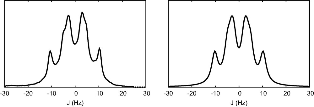
The multiplet at δ = 3.81 ppm (TMS as reference) in the ¹H NMR spectrum of sucrose dissolved in perdeuterated DMSO (left). The multiplet that is reconstructed from the AUJ analysis, with J = 5.37 Hz, 7.04 Hz, 8.14 Hz and $T_{2}^{*}$ = 0.1 s (right).

The 1-D J-spectrum is analyzed as J = 1.47 Hz (0.55), 2.13 Hz (0.54), 5.57 Hz (1.32), 7.20 Hz (0.72), and 8.25 Hz (0.80), where numbers in parenthesis are the $\bar{n}$ non-integer multiplicity values. Multiplicity refinement eliminates the two lowest J values and proposes the remaining ones to correspond to doublets. This behavior is very common, as the not strictly Lorentzian peak shape may be seen by the algorithm as originating from small, non-resolved coupling constants. The final refinement of the J values produces three close but different coupling constants: J = 5.37 Hz, 7.04 Hz, and 8.14 Hz, giving rise to a reconstructed multiplet that is very similar to the original one (Fig. 1, right).

A more difficult problem was given to AUJ, the analysis of a multiplet that is simulated on the basis of results presented in [11] for the methine proton of 3-bromo-2-methyl-1-propanol (Fig. 2, left). The multiplet is a quadruplet of quintet with J = 5.43 Hz and 6.76 Hz, respectively. Some computer generated noise is added to the spectrum and the line width is chosen so that peak clusters are poorly resolved. The 1-D J-spectrum is interpreted as J = 1.10 Hz (0.77), 5.46 Hz (1.24), and 6.69 Hz (1.80). Again, the noise introduces unwanted small coupling constants in the 1-D J-spectrum. The multiplicity optimization step finds the correct result and the final refinement produces J₁ = 5.39 Hz, J₂ = 5.40 Hz, J₃ = 5.41 Hz, J₄ = J₅ = J₆ = 6.78 Hz, J₇ = 6,79 Hz, a result that compares well to what is expected.

Fig. 2
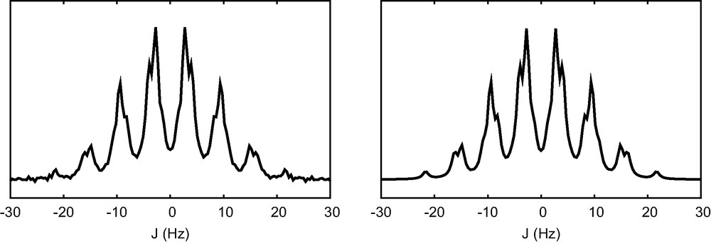
Experiment on simulated data, using parameters published in [11] for the methine proton of 3-bromo-2 methyl-1-propanol. Simulated spectrum, using J₁ = J₂ = J₃ = 5.43 Hz, J₄ = J₅ = J₆ = J₇ = 6.76 Hz and $T_{2}^{*}$ = 0.25 s. Some computer-generated Gaussian noise was added (left). The multiplet that was reconstructed from the AUJ analysis, with J₁ = 5.39 Hz, J₂ = 5.40 Hz, J₃ = 5.41 Hz, J₄ = J₅ = J₆ = 6.78 Hz, J₇ = 6,79 Hz, and T = 0.254 s (right).

4 Conclusion

This Communication shows that the AUJ algorithm provides a pertinent way to analyze complex multiplets. The modeling of time-domain data ensures a reliable result on poorly resolved signals, even though non-ideal lineshapes and high noise levels may lead the user to modify the default algorithm parameters. However, it should always been remembered that the best first order analysis algorithm ever written cannot provide a safe and useful result if carried out on a part of a strongly coupled spin system. Further development of AUJ will deal with parameter selection improvement, the interfacing of the algorithm with commercial NMR data processing software, as well as its extension to slices of 2-D NMR spectra, different from J-resolved ones, in order to analyze nearly or fully superimposed multiplets.

Acknowledgements

We thank Dr. Karen Plé for linguistic improvement.