

1 Introduction
Accurate prediction of thermodynamic properties of fluids and phase equilibrium in mixtures is required for the design and simulation of industrial processes. In particular, processes involved in petroleum production from natural hydrocarbon reserves require good representation of the phase behavior in different type of mixtures. In describing phase equilibrium, equations of state (EoS) have been commonly employed and numerous models are available in the literature [1]. In specific applications, however, some EoS are not of sufficient accuracy, mainly because of inadequate use of the mixing rules [1–3]. That is mainly the reason of the very limited use of EoS for describing properties of mixtures containing polar substances that self-associate through hydrogen bonding (such as water or alcohols).
Kretschmer and Wiebe [4] presented an interesting study on the thermodynamics of alcohol + hydrocarbon mixtures but they did not discuss the vapor-liquid equilibrium (VLE) in these mixtures. For VLE calculations, several approaches have been proposed to account for the association in this type of mixtures. Hanks et al. [5] used the continuous linear association model (CLAM) to predict vapor-liquid equilibrium of thirty-five binary mixtures alcohol + aromatic hydrocarbons. The authors found that the model properly represented the large deviations from ideal solutions that arise from alcohol association. Yakoumis et al. [6] used the so-called Cubic-Plus-Association equation of state (CPA-EoS) to study binary systems containing one associating compound (alcohol) and an inert one (hydrocarbon). The CPA-EoS combines the Soave-Redlich-Kwong equation (SRK) for the physical part with an association term based on perturbation theory. The authors found better results than those obtained by the SRK equation and its performance was similar to that of other association models, such as the Anderko EoS, and the more complex SAFT and Simplified SAFT-EoS. Pires et al. [2] considered an EoS formed by two contributions (physical and chemical) as proposed by Anderko [7], and correlated bubble point pressure data for binary water + hydrocarbon and alcohol + hydrocarbon systems. The results obtained were in reasonable agreement with the experimental data. Li and Englezos [8] employed the SAFT-EoS to correlate phase equilibrium in systems containing alcohols, water, carbon dioxide and hydrocarbons. They considered eighteen systems of which six are alcohol + hydrocarbon mixtures. Good results were found for the vapor phase concentration but higher deviations were found for the bubble pressure. Dell’ Era et al. [9] determined VLE data for the systems butane + alcohols and used several liquid phase models and COSMO-RS for correlating the experimental data. Al-Saifi et al. [10] applied the dipolar PC-SAFT to correlate and predict phase equilibrium of alcohol + hydrocarbon mixtures using three dipolar terms. The results were in good agreement with experimental data, although for several systems the authors did not report deviations for the vapor phase concentrations.
Most of the models presented above require several pure component parameters that are obtained by fitting experimental data (usually vapor pressure data) and also contain some binary interaction parameters obtained from binary VLE data. This makes the models more difficult to use in comparison with classical EoS in which the critical properties, easily found in the open literature, are usually employed. For instance, the application of the complex EoS for associating fluids presented by Pires et al. [2] requires the energy and entropy of vaporization of each component in the mixture, values determined by fitting vapor pressure and liquid density data. Also, other parameters claimed by the authors to be available are not easily found for many substances (characteristic temperature of intermolecular interactions, characteristic molar volume and external degrees of freedom of a molecule). Additionally, the model requires three adjustable parameters for binary mixtures. Al-Saifi et al. [10] applied the dipolar PC-SAFT claiming that good results were found with no adjustable parameters for binary mixtures. However, they had to fit six pure component parameters for each of the component in the mixture (12 parameters per binary mixture) to get the alleged good results. Yakoumis et al. [6] use the CPA equation of state with five adjustable parameters for each component in the mixture (10 parameters per binary mixture).
To correlate VLE data for this type of mixtures, classical equations of state with modern mixing rules usually require few adjustable parameters. Among the several models of this type available in the literature the Peng-Robinson EoS with the Wong-Sandler mixing rules including the van Laar model for the activity coefficient (PR/WS/VL model with three adjustable parameters) have demonstrated to have the necessary flexibility for representing in acceptable form the phase behavior of complex mixtures [11]. It seems that the three adjustable parameters of the PR/WS/VL model are able to take into account all the different factors that affect phase behavior in these types of mixtures. To the best of the authors’ knowledge this is the first time that a systematic study on the application of the PR/WS/VL model to associating alcohol + hydrocarbon mixtures has been successfully done.
The Table 1 shows the characteristics of several models that have been applied to alcohols + hydrocarbons mixtures. The very different characteristics of the various models should be considered when the goodness of a model is compared with the results of other researchers that use models with different characteristics. The following factors must be considered to decide which is the best model for a given application:
- • the mathematical complexity of the model;
- • the type and amount of basic properties used by the model;
- • the number of adjustable pure component parameters;
- • the number of adjustable binary interaction parameters;
- • the physical meaning of the parameters;
- • the range of applicability (pressure and temperature) and;
- • the generalization of the model (type of fluids and mixtures).
Main characteristics of various models presented in the literature for correlating VLE data of alkane + alcohol mixtures.
| Author/model | Mixtures studied | Pure component parameters | Interaction parameters | Objective function | Comments |
| Yakoumis et al. (1997) [6] CPA-EoS | Alcohols + hydrocarbons | 5 (adjustable) | 1 (adjustable from VLE data) | The five pure component parameters for each compound in the mixture are determined from regression of vapor pressure and density data | |
| Pires et al. (2001) [2] Anderko-EoS | Alcohols + hydrocarbons | 6 (3 adjustable and 3 from literature) | 1 (adjustable from VLE data) | Two of the pure component parameters for each compound in the mixture are determined from regression of vapor pressure and density data. The other parameters are claimed to be found in the literature but are not readily available | |
| Li and Englezos (2004) [8] SAFT-EoS | Alcohols, water, carbon dioxide with hydrocarbons | 5 for alcohols components and 3 for hydrocarbons (all adjustable) | 2 (adjustable from VLE data) | Not reported | Five pure component parameters for alcohols components and three parameters for hydrocarbons are required. These parameters are estimated by regression of saturated vapor pressure and liquid density data |
| Al-Saifi et al. (2008) [10] PC-SAFT-JC | Water + alcohols, hydrocarbons; alcohols + alcohols, hydrocarbons. | 6 (adjustable) | None | Not reported | PC-SAFT-JC requires six adjustable parameters when considering associating components determined by regression of vapor pressure and liquid density |
| This Work PR/WS/VL EoS | Alcohols + hydrocarbons | 3 (from the literature) | 3 (adjustable from VLE data) | The three pure component parameters (critical temperature, critical pressure and acentric factor) are readily available in the open literature. The three parameters for the mixture are obtained from VLE data |
The best model should be that which appropriately compensates physical foundation, accuracy of the results and mathematical simplicity. These concepts are applied in this paper to compare the results of the model employed with other results from the literature.
2 The thermodynamic model
Of the many equations of state nowadays available, the so-called cubic equations derived from van der Waals proposal such as the Peng-Robinson EoS [12], are widely used to treat a wide variety of mixtures. The EoS proposed by Peng and Robinson can be written in a general form as follows:
| (1) |
In this equation, a and b are parameters, specific for each substance, determined using the critical properties, Tc and Pc, and the temperature for “a”. Commonly a = acα(TR).
| (2) |
F = 0.37464 + 1.54226 ω − 0.26992 ω2
For mixtures the EoS parameters (a and b) are replaced by mixtures parameters (am y bm):
| (3) |
In this work, the Wong-Sandler (WS) mixing rules has been used to express the dependency of the parameters am y bm on concentration. The WS mixing rules for the Peng-Robinson EoS can be summarized as follows [13]:
| (4) |
In these equations, kij is an interaction parameter, Ω = −0.62323 for the Peng-Robinson EoS, and A∞E(y) is calculated assuming that A∞E(y) ≈ A0E(y) ≈ g0E, being g0E the excess Gibbs free energy. For g0E several models have been used in the literature. In this work g0E has been calculated using the van Laar model:
| (5) |
In the equations (4) and (5) “x” represents the mole fraction in the liquid phase when the fugacity coefficient for the components in the liquid phase is determined, and “x” represents the mole fraction in the vapor phase when the fugacity coefficient for the components in the vapor phase is calculated.
For a binary mixture the WS mixing rule includes one adjustable binary interaction parameter k12 for (b-a/RT)ij, besides the two parameters, A12 and A21, included in the g0E model. These three adjustable parameters for each of the mixtures have been determined using experimental phase equilibrium data at constant temperature, available in the literature. In summary, the thermodynamic model used in this work includes the Peng-Robinson equation of state, the Wong-Sandler mixing rule, and the van Laar model for g0E in the mixing rules, and contains three adjustable parameters. The model is designated as PR/WS/VL in the rest of the paper.
3 Mixtures Studied
Twenty-four binary alcohol + hydrocarbon mixtures were considered in this study. The alcohols included in the mixtures are: methanol, ethanol, 1-propanol, 2-propanol and 2-butanol and the hydrocarbons considered are: methane, ethane, propane, n-butane, n-pentane, n-hexane and n-heptane. Table 2 shows pure component properties for all the substances involved in this study. In the table, M is the molecular mass, Tb is the normal boiling temperature, Tc is the critical temperature, Pc is the critical pressure, Vc is the critical volume and ω is the acentric factor. The values for these properties were obtained from Daubert et al. [14].
Properties for all substances involved in this study.
| Components | M (kg/kg mol) | Tb (K) | Tc (K) | Pc (bar) | Vc (m3/kmol) | ω |
| Alkanols | ||||||
| methanol | 32.0 | 337.85 | 512.65 | 80.84 | 0.117 | 0.5659 |
| ethanol | 46.1 | 351.45 | 513.95 | 61.37 | 0.168 | 0.6436 |
| 1-propanol | 60.1 | 370.35 | 536.75 | 51.69 | 0.218 | 0.6204 |
| 2-propanol | 60.1 | 355.41 | 508.30 | 47.64 | 0.222 | 0.6669 |
| 2-butanol | 74.1 | 372.70 | 536.20 | 42.02 | 0.269 | 0.5768 |
| Hydrocarbons | ||||||
| methane | 16.0 | 111.66 | 190.56 | 45.99 | 0.099 | 0.0116 |
| ethane | 30.1 | 184.55 | 305.32 | 48.72 | 0.146 | 0.0995 |
| propane | 44.1 | 231.11 | 369.83 | 42.48 | 0.200 | 0.1523 |
| n-butane | 58.1 | 272.65 | 425.12 | 37.96 | 0.255 | 0.2002 |
| n-pentane | 72.2 | 309.22 | 469.70 | 33.70 | 0.313 | 0.2515 |
| n-hexane | 86.2 | 341.88 | 507.60 | 30.25 | 0.371 | 0.3013 |
| n-heptane | 100.2 | 371.58 | 540.20 | 27.40 | 0.428 | 0.3495 |
Table 3 gives some details on the experimental data used in the study including the literature source for each data set. In this table, T is the temperature (expressed in kelvin), n is the number of experimental data, x1 is the liquid mole fraction for component 1, y1 is the vapor mole fraction for component 1 and P is the pressure (expressed in bars). As seen in Table 3, data for 70 isotherms with a total of 700 data points were considered. The temperature ranges from 298 to 523 K and the pressure from about 0.5 to 105 bars.
Details on the phase equilibrium data for the systems considered in this study. In the table the temperature values have been rounded to the closest integer.
| Systems | References | T (K) | N | Range of data | ||
| Range of x1 | Range of y1 | Range of P (bar) | ||||
| Methanol (2) + | ||||||
| Ethane (1) | Ishira et al. [21] | 298 | 7 | 0.053–0.988 | 0.959–0.998 | 9.63–41.55 |
| Courtial et al. [22] | 323 | 11 | 0.069–0.973 | 0.841–0.938 | 3.37–5.28 | |
| Dell Era et al. [9] | 364 | 25 | 0.009–0.999 | 0.268–0.968 | 3.69–14.41 | |
| Propane (1) | Leu et al. [23] | 311 | 11 | 0.016–0.984 | 0.822–0.980 | 2.12–13.43 |
| 352 | 8 | 0.020–0.975 | 0.660–0.966 | 5.60–31.73 | ||
| 393 | 8 | 0.027–0.589 | 0.502–0.764 | 14.46–57.32 | ||
| 474 | 6 | 0.028–0.173 | 0.146–0.274 | 53.01–86.63 | ||
| n-Butane (1) | Courtial et al. [22] | 373 | 13 | 0.018–0.988 | 0.368–0.965 | 5.72–17.20 |
| 403 | 11 | 0.019–0.992 | 0.248–0.982 | 11.75–30.91 | ||
| 423 | 7 | 0.019–0.713 | 0.226–0.735 | 19.64–43.74 | ||
| 433 | 11 | 0.009–0.424 | 0.103–0.615 | 20.82–48.45 | ||
| 443 | 7 | 0.011–0.369 | 0.067–0.504 | 24.54–54.34 | ||
| Leu et al. [23] | 470 | 5 | 0.008–0.261 | 0.039–0.261 | 40.11–69.17 | |
| n-Pentane (1) | Wilsak et al. [24] | 373 | 9 | 0.012–0.956 | 0.224–0.795 | 4.51–8.46 |
| 398 | 9 | 0.045–0.975 | 0.298–0.888 | 10.44–15.12 | ||
| 423 | 9 | 0.033–0.940 | 0.187–0.819 | 16.91–25.28 | ||
| Ethanol (2) + | ||||||
| Methane (1) | Suzuki et al. [15] | 313 | 5 | 0.021–0.107 | 0.989–0.994 | 18.08–100.73 |
| 333 | 5 | 0.028–0.105 | 0.977–0.989 | 25.94–104.64 | ||
| Ethane (1) | Suzuki et al. [15] | 313 | 5 | 0.078–0.602 | 0.984–0.992 | 13.65–54.14 |
| 333 | 9 | 0.057–0.567 | 0.958–0.981 | 13.07–78.97 | ||
| Propane (1) | Zabaloy et al. [17] | 325 | 6 | 0.169–0.881 | 0.974–0.988 | 9.74–18.00 |
| 350 | 5 | 0.160–0.858 | 0.935–0.973 | 13.57–29.60 | ||
| 375 | 5 | 0.171–0.837 | 0.874–0.943 | 20.19–43.81 | ||
| n-Butane (1) | Soo et al. [16] | 323 | 9 | 0.193–0.974 | 0.919–0.970 | 3.81–5.03 |
| 353 | 9 | 0.109–0.962 | 0.782–0.952 | 5.61–10.34 | ||
| 373 | 12 | 0.025–0.976 | 0.428–0.965 | 4.26–15.72 | ||
| 403 | 10 | 0.035–0.973 | 0.353–0.965 | 9.51–20.73 | ||
| 423 | 14 | 0.027–0.975 | 0.210–0.973 | 13.25–38.00 | ||
| n-Pentane (1) | Seo et al. [18] | 423 | 9 | 0.059–0.904 | 0.242–0.840 | 12.79–19.68 |
| 465 | 13 | 0.079–0.979 | 0.172–0.974 | 31.00–41.45 | ||
| 500 | 5 | 0.018–0.120 | 0.033–0.120 | 50.30–57.19 | ||
| n-Hexane (1) | Seo et al. [19] | 473 | 12 | 0.013–0.959 | 0.025–0.887 | 20.16–34.79 |
| 483 | 11 | 0.032–0.951 | 0.046–0.880 | 23.76–40.99 | ||
| 493 | 10 | 0.025–0.937 | 0.026–0.902 | 28.13–48.85 | ||
| 503 | 5 | 0.016–0.954 | 0.018–0.954 | 31.04–55.61 | ||
| n-Heptane (1) | Seo et al. [20] | 483 | 10 | 0.051–0.896 | 0.059–0.793 | 17.20–36.77 |
| 508 | 11 | 0.027–0.859 | 0.030–0.753 | 26.17–56.58 | ||
| 523 | 5 | 0.721–0.910 | 0.721–0.852 | 27.95–37.72 | ||
| 1-Propanol (2) + | ||||||
| Methane (1) | Suzuki et al. [15] | 313 | 5 | 0.036–0.141 | 0.996–0.998 | 21.65–100.79 |
| 333 | 5 | 0.020–0.130 | 0.985–0.994 | 14.10–101.97 | ||
| Ethane (1) | Suzuki et al. [15] | 313 | 5 | 0.106–0.547 | 0.994–0.996 | 13.47–51.11 |
| 333 | 6 | 0.080–0.503 | 0.971–0.991 | 13.56–67.42 | ||
| Propane (1) | Jiménez-Gallegos et al. [26] | 318 | 9 | 0.139–0.665 | 0.988–0.995 | 5.75–13.14 |
| 324 | 8 | 0.111–0.871 | 0.983–0.994 | 5.28–15.71 | ||
| 349 | 8 | 0.097–0.940 | 0.948–0.989 | 5.40–26.41 | ||
| n-Butane (1) | Panasen et al. [25] | 330 | 24 | 0.012–0.988 | 0.631–0.994 | 0.47–5.90 |
| n-Pentane (1) | Jung et al. [27] | 468 | 15 | 0.020–0.948 | 0.064–0.946 | 16.79–33.52 |
| 483 | 13 | 0.026–0.592 | 0.072–0.592 | 22.39–40.29 | ||
| 498 | 10 | 0.020–0.415 | 0.042–0.415 | 28.64–44.45 | ||
| 513 | 7 | 0.025–0.245 | 0.047–0.245 | 37.26–48.24 | ||
| 2-Propanol (2) + | ||||||
| Ethane (1) | Kodama et al. [28] | 308 | 9 | 0.260–0.990 | 0.990–0.996 | 21.91–49.90 |
| 313 | 8 | 0.336–0.978 | 0.984–0.996 | 31.69–53.57 | ||
| Propane (1) | Zabaloy et al. [30] | 333 | 8 | 0.094–0.902 | 0.920–0.994 | 5.70–19.82 |
| n-Butane (1) | Moilanen et al. [29] | 323 | 23 | 0.031–0.986 | 0.713–0.986 | 0.81–4.95 |
| n-Hexane (1) | Seo et al. [31] | 483 | 14 | 0.029–0.904 | 0.042–0.878 | 24.31–33.76 |
| 493 | 18 | 0.040–0.935 | 0.045–0.924 | 26.80–39.85 | ||
| 503 | 9 | 0.022–0.973 | 0.027–0.970 | 29.45–45.46 | ||
| n-Heptane (1) | Oh et al. [32] | 483 | 11 | 0.039–0.908 | 0.039–0.853 | 15.14–31.21 |
| 498 | 11 | 0.039–0.882 | 0.039–0.806 | 19.70–40.21 | ||
| 508 | 7 | 0.410–0.892 | 0.410–0.837 | 22.45–39.67 | ||
| 523 | 6 | 0.725–0.898 | 0.725–0.848 | 26.79–34.17 | ||
| 2-Butanol (2) + | ||||||
| Propane (1) | Gros et al. [33] | 328 | 11 | 0.286–0.995 | 0.987–0.999 | 10.10–18.97 |
| 348 | 11 | 0.286–0.995 | 0.973–0.998 | 13.65–28.24 | ||
| 368 | 11 | 0.274–0.995 | 0.946–0.997 | 17.03–40.82 | ||
| n-Butane (1) | Moilanen et al. [29] | 323 | 23 | 0.027–0.99 | 0.797–0.997 | 0.52–4.92 |
| Dell Era et al. [9] | 364 | 25 | 0.016–0.989 | 0.399–0.995 | 1.24–12.74 | |
| n-Pentane (2) | Kim et al. [34] | 468 | 12 | 0.064–0.977 | 0.147–0.977 | 15.88–32.72 |
| 483 | 11 | 0.042–0.706 | 0.097–0.706 | 19.39–36.80 | ||
| 498 | 9 | 0.033–0.495 | 0.060–0.495 | 25.01–39.06 | ||
| 513 | 6 | 0.049–0.301 | 0.079–0.301 | 31.62–40.94 |
Bubble pressure calculations for binary mixtures were performed using the PR/WS/VL model. The adjustable parameters of the model (k12, A12, A21) were determined by optimization of the objective function given by eqn. (6). The program designed considers the use of the Levenberg-Marquardt algorithm as the optimization method [35]. The objective function was defined as the relative error between calculated and experimental values of the pressure:
| (6) |
In this equation N is the number of points in the experimental data set and P is the bubble pressure.
4 Results and discussion
Table 4 shows the optimum binary interaction parameters in the Wong-Sandler mixing rule at all temperatures studied and the results for the pressure P and the vapor mole fraction y1 for the 24 binary mixtures. This table shows the average-absolute deviations for the pressure ǀ%ΔPǀ, and the average-absolute deviations and average-relative deviations for the concentration of component 1 in the vapor phase ǀ%Δy1ǀand %Δy1, respectively. For a set of N data these deviations are defined as follows:
| (7) |
Optimum binary interaction parameter and van Laar constants in the Wong-Sandler mixing rules at all temperatures studied and average deviations for the pressure and vapor mole fraction of component (1), using the PR/WS/VL model.
| Systems | T (K) | A12 | A21 | k12 | ǀ% ΔPǀ | ǀ%Δy1ǀ | %Δy1 |
| Methanol (2) + | |||||||
| Ethane (1) | 298 | 1.5133 | 1.4666 | 0.1079 | 2.3 | 0.7 | 0.5 |
| Propane (1) | 311 | 1.4379 | 0.4262 | 0.5323 | 5.1 | 1.7 | 1.7 |
| 352 | 1.2473 | 0.4211 | 0.5154 | 4.9 | 2.3 | 2.3 | |
| 393 | 1.8014 | 0.7234 | 0.4019 | 2.5 | 6.6 | 2.2 | |
| 474 | 2.5750 | 2.1315 | 0.1336 | 0.4 | 1.2 | 0.4 | |
| n-Butane (1) | 323 | 2.6762 | 3.6923 | 0.0514 | 4.9 | 1.6 | 0.6 |
| 364 | 2.5154 | 3.9707 | 0.0882 | 3.8 | 2.6 | −0.9 | |
| 373 | 2.3601 | 3.0773 | 0.2148 | 4.5 | 2.4 | 1.7 | |
| 403 | 1.9084 | 2.3213 | 0.3157 | 2.8 | 1.8 | 0.6 | |
| 423 | 2.0916 | 1.2503 | 0.3562 | 3.7 | 3.4 | 2.0 | |
| 433 | 2.3232 | 1.5134 | 0.3081 | 2.8 | 2.8 | < 0.1 | |
| 443 | 2.3487 | 3.9115 | 0.1396 | 2.5 | 6.5 | −4.0 | |
| 470 | 2.6143 | 2.4354 | 0.1624 | 0.7 | 1.6 | < 0.1 | |
| n-Pentane (1) | 373 | 2.7736 | 3.6646 | 0.1569 | 3.8 | 6.5 | −4.7 |
| 398 | 2.3332 | 3.5473 | 0.1894 | 1.7 | 2.9 | −1.1 | |
| 423 | 1.6295 | 3.2400 | 0.3209 | 1.1 | 4.2 | 0.4 | |
| Ethanol (2) + | |||||||
| Methane (1) | 313 | 0.9632 | 1.3324 | 0.0339 | 0.7 | 0.3 | −0.3 |
| 333 | 0.9312 | 1.4921 | 0.0886 | 0.3 | 0.4 | −0.4 | |
| Ethane (1) | 313 | 1.3525 | 1.1306 | 0.1385 | 3.6 | 1.9 | −1.9 |
| 333 | 1.3535 | 1.1249 | 0.1585 | 2.5 | 0.7 | −0.7 | |
| Propane (1) | 325 | 1.1841 | 3.6667 | 0.1274 | 3.6 | 0.9 | −0.9 |
| 350 | 1.0263 | 3.8665 | 0.1266 | 3.1 | 1.6 | −1.6 | |
| 375 | 1.0471 | 3.2831 | 0.1235 | 2.6 | 3.8 | −3.8 | |
| n-Butane (1) | 323 | 1.77830 | 3.7293 | 0.0581 | 2.6 | 0.6 | −0.4 |
| 353 | 2.0813 | 3.7653 | 0.0109 | 1.6 | 0.9 | −0.6 | |
| 373 | 2.1273 | 3.7560 | 0.0064 | 2.5 | 1.6 | < 0.1 | |
| 403 | 2.0774 | 3.3002 | 0.0491 | 1.4 | 1.4 | 0.7 | |
| 423 | 2.0032 | 3.2235 | 0.0704 | 1.1 | 3.4 | −1.9 | |
| n-Pentane (1) | 423 | 2.0574 | 2.5842 | 0.1176 | 0.4 | 1.3 | 0.4 |
| 465 | 2.1698 | 3.0782 | 0.0496 | 0.9 | 1.9 | −1.0 | |
| 500 | 1.7118 | 1.5856 | 0.1850 | 0.5 | 2.7 | −2.5 | |
| n-Hexane (1) | 473 | 1.6305 | 1.5880 | 0.2202 | 0.4 | 3.9 | 3.7 |
| 483 | 0.9195 | 1.6116 | 0.2855 | 1.4 | 3.6 | 3.5 | |
| 493 | 0.1563 | 0.1008 | 0.2154 | 1.9 | 2.3 | 1.5 | |
| 503 | 0.9101 | 0.8509 | 0.2405 | 1.1 | 2.0 | 1.5 | |
| n-Heptane (1) | 483 | 2.3865 | 2.1708 | 0.1194 | 1.0 | 4.0 | −2.5 |
| 508 | 1.4868 | 1.5011 | 0.2698 | 0.8 | 1.6 | −1.3 | |
| 523 | 0.4651 | 2.2526 | 0.3496 | 0.8 | 1.0 | −0.6 | |
| 1-Propanol (2) + | |||||||
| Methane (1) | 313 | 0.5417 | 2.4752 | 0.0952 | 2.8 | 0.2 | −0.2 |
| 333 | 0.6396 | 1.0645 | 0.1599 | 0.7 | 0.3 | −0.3 | |
| Ethane (1) | 313 | 0.8963 | 1.5307 | 0.0709 | 0.4 | 0.3 | −0.3 |
| 333 | 0.9330 | 1.4436 | 0.0739 | 0.2 | 0.6 | −0.6 | |
| Propane (1) | 318 | 0.8108 | 0.6629 | 0.2771 | 0.8 | 0.4 | −0.4 |
| 324 | 0.7694 | 0.5676 | 0.2983 | 0.8 | 0.5 | −0.5 | |
| 349 | 0.2286 | 0.2342 | 0.3253 | 2.0 | 0.7 | −0.7 | |
| n-Butane (1) | 330 | 1.4574 | 3.2947 | 0.0410 | 2.3 | 1.0 | −1.0 |
| n-Pentane (1) | 468 | 1.1738 | 2.0650 | 0.1053 | 1.5 | 6.8 | 6.5 |
| 483 | 1.0540 | 1.9969 | 0.1227 | 1.2 | 2.8 | 1.0 | |
| 498 | 1.2374 | 1.2503 | 0.1217 | 0.6 | 5.8 | 3.8 | |
| 513 | 1.0424 | 1.3454 | 0.1526 | 0.5 | 1.4 | −0.3 | |
| 2-Propanol (2) + | |||||||
| Ethane (1) | 308 | 2.0846 | −0.1849 | 0.1715 | 1.1 | 0.7 | −0.6 |
| 313 | 1.4134 | −0.2152 | 0.1600 | 2.3 | 0.5 | −0.3 | |
| Propane (1) | 333 | 1.8783 | 0.2539 | 0.3968 | 3.4 | 0.6 | 0.1 |
| n-Butane (1) | 323 | 1.4622 | 3.1920 | 0.0427 | 2.2 | 1.0 | −0.6 |
| 483 | 0.8971 | 1.0537 | 0.1867 | 0.3 | 3.1 | −1.1 | |
| n-Hexane (1) | 493 | 1.4450 | 1.3889 | 0.0829 | 0.6 | 2.1 | 0.8 |
| 503 | 0.1437 | 2.3500 | 0.3168 | 0.7 | 2.8 | 0.4 | |
| n-Heptane (1) | 483 | 1.5888 | 1.7465 | 0.0855 | 1.3 | 5.0 | −2.5 |
| 498 | 1.1498 | 1.0290 | 0.1707 | 0.3 | 4.2 | −1.5 | |
| 508 | 1.3576 | 0.8700 | 0.1741 | 0.7 | 2.4 | −2.2 | |
| 523 | 1.3850 | 0.7724 | 0.1767 | 1.0 | 0.6 | −0.4 | |
| 2-Butanol (2) + | |||||||
| Propane (1) | 328 | 1.2356 | 0.3856 | 0.3182 | 0.9 | 0.2 | −0.1 |
| 348 | 1.1224 | 0.4155 | 0.2730 | 0.5 | 0.2 | −0.1 | |
| 368 | 0.7374 | 0.4868 | 0.2165 | 0.2 | 0.1 | < 0.1 | |
| n-Butane (1) | 323 | 1.2424 | 2.8698 | 0.0128 | 1.6 | 1.1 | −1.1 |
| 364 | 1.1162 | 2.5751 | 0.0289 | 1.1 | 1.0 | −0.9 | |
| 468 | 1.2446 | 1.4554 | 0.0084 | 1.0 | 9.2 | 9.1 | |
| n-Pentane (2) | 483 | 1.0224 | 1.5354 | 0.0255 | 0.9 | 5.8 | 3.2 |
| 498 | −0.0624 | −0.0940 | 0.1535 | 5.2 | 7.9 | 3.4 | |
| 513 | 0.5970 | 2.8956 | 0.1002 | 0.6 | 1.3 | 0.4 |
As seen in Table 4, the PR/WS/VL model reproduces the bubble pressures of these binary mixtures with mean absolute deviations less than 5.3% for any temperature. The pressure was calculated with deviations between 0.3% and 5.2%. Of the seventy studied isotherms, 27 are reproduced with deviations less than 1%, 31 with deviations from 1.0% to 3.0%, 7 with deviations from 3.1% to 4.0%, and 5 with deviations from 4.1% to 5.2%.
With respect to the hydrocarbon concentration in the vapor phase y1, this quantity is predicted in all cases with average-absolute deviations from 0.3% to 9.2%. Of the seventy studied isotherms, 21 are reproduced with deviations less than 1%, 38 with deviations from 1.0% to 4.0%, 5 with deviations from 4.1% to 6.0%, 5 with deviations from 6.1% to 8.0%, and 1 with the maximum deviation found (9.2%). The average-relative deviations vary between −3.8% and 9.1%.
The Table 5 shows results for similar mixtures presented by Yakoumis et al. [6], Pires et al. [2], Li and Englezos [8] and Al-Saifi et al. [10] with the models described in Table 1 and with results of Soo et al. [16] and Courtial et al. [22] who used the PR equation of state with the Wong-Sandler mixing rules but including the NRTL model for the excess Gibbs free energy instead of the van Laar model used in the present paper (PR/WS/NRTL). In the overall, results are similar. Thus, by only analyzing the average deviations, none of the models shows superiority over the others. In the average, the complex literature models correlate pressure with 2.1% absolute deviations and our model with 2.4%. The concentration of the hydrocarbon in the gas phase is correlated with other models with average-absolute deviations of 3.5% while the PR/WS/VL model gives a little lower value (3.0% in the average).
Comparison between this work and results from the literature for same alcohol + hydrocarbon mixtures using different models. The indexes a y b indicate that the values were determined using other deviations definitions as given at end of the table.
| Mixture | References/model | T (K) | ǀ%ΔPǀ | ǀ%Δy1ǀ | ǀ% ΔPǀ | ǀ%Δy1ǀ |
| This work | ||||||
| Butane (1) + ethanol (2) | Yakoumis et al. [6]/CPA | 323 | 2.0 | ---- | ||
| Li and Englezos [8]/SAFT | 19.9a | 0.0082b | 2.6 | 0.6 | ||
| Al-Saifi et al. [10]/PC-SAFT | 2.1 | ---- | ||||
| Seo et al. [16]/PR/WS/NRTL | ---- | 0.2 | ||||
| 353 | ---- | 0.8 | 1.6 | 0.9 | ||
| 373 | ---- | 1.2 | 2.5 | 1.6 | ||
| 403 | ---- | 1.5 | 1.4 | 1.4 | ||
| 423 | ---- | 6.7 | 1.1 | 3.4 | ||
| n-pentane (1) + methanol (2) | Yakoumis et al. [6]/CPA | 373 | 2.0 | 1.7 | 3.8 | 6.5 |
| 398 | 1.8 | 1.7 | 1.7 | 2.9 | ||
| 423 | 2.2 | 1.3 | 1.1 | 4.2 | ||
| Butane (1) + methanol (2) | Pires et al. [2]/Anderko EoS | 323 | 4.2 | 11.3 | 4.9 | 1.6 |
| Courtial et al. [22]/PR/WS/NRTL | ---- | 0.6 | ||||
| 373 | ---- | 1.6 | 4.5 | 2.4 | ||
| 403 | ---- | 2.5 | 2.8 | 1.8 | ||
| 423 | ---- | 4.8 | 3.7 | 3.4 | ||
| 433 | ---- | 9.2 | 2.8 | 2.8 | ||
| 443 | ---- | 16.1 | 2.5 | 6.5 | ||
| n-Pentane (1) + methanol (2) | Wilsak et al. [24] | 373 | 2.9 | 6.8 | 3.8 | 6.5 |
| 398 | 1.0 | 5.5 | 1.7 | 2.9 | ||
| 423 | 0.6 | 4.0 | 1.3 | 3.3 | ||
| n-pentane (1) + methanol (2) | Al-Saifi et al. [10]/PC-SAFT | 373 | 2.3 | 1.1 | 3.8 | 6.5 |
| 398 | 2.5 | 0.7 | 1.7 | 2.9 | ||
| 423 | 2.8 | 0.4 | 1.3 | 3.3 | ||
| n-pentane (1) + ethanol (2) | Soo et al. [18] | 423 | 1.7 | 0.2 | 0.4 | 1.3 |
| 465 | 1.0 | 0.1 | 0.9 | 1.9 | ||
| Propane (1) + ethanol (2) | Li and Englezos [8]/SAFT | 325 | 12.2a | 0.0176b | 3.6 | 0.9 |
| 350 | 14.6a | 0.0221b | 3.1 | 1.6 |
a
b
As explained in the Introduction section comparison between different models must considered several factors besides its accuracy. Considering the characteristics of the PR/WS/VL model such as: the number and availability of basic properties used by the model (critical properties and acentric factor only), the number of adjustable parameters for the mixtures (three for binary mixtures), the wide range of applicability (pressure and temperature), the equations used in this work represents an acceptable model giving results with accuracy similar to more sophisticated equations that use several pure component properties that are frequently not available.
As additional examples of the results provided by the PR/WS/VL model, the Figs. 1–3 show the bubble pressure versus concentration for three mixtures with different behavior. The Fig. 1 shows results for the mixture ethane (1) + ethanol (2) at 333 K, in which one of the components is much more volatile than the other so the concentration of component 1 in the vapor phase is much higher than in the liquid phase especially at low pressures. The Fig. 2 shows results for the mixture n-pentane (1) + 1-propanol (2) at 498 K, in which both components have similar volatilities so the concentration of component 1 in the vapor phase is similar to that of the liquid phase at all pressures. The Fig. 3 shows results for the mixture n-butane (1) + methanol (2) at 443 K, which shows an intermediate behavior as those presented in Figs. 1 and 2. In the figures, the symbol (●) represents the experimental data and the dashed line (---) represents the calculated values. It can be seen that there is good agreement between model estimates and experimental data in both cases, showing the versatility of the model.
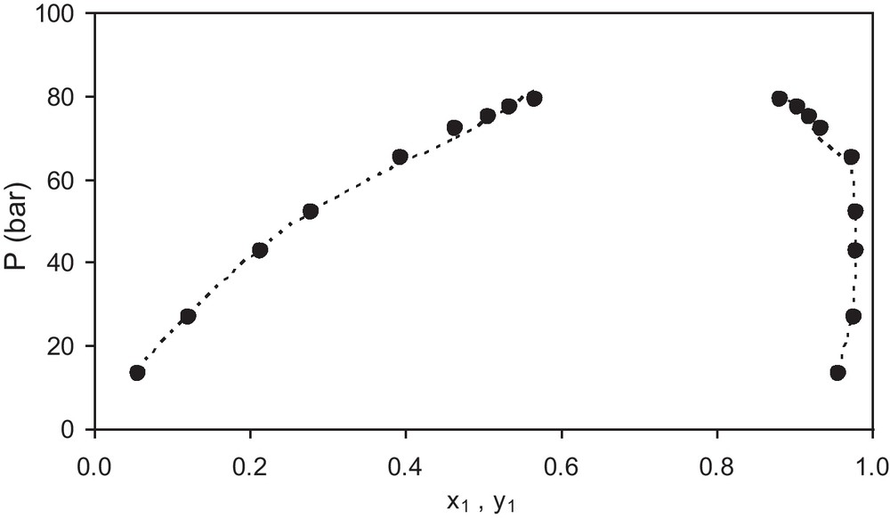
Experimental (●) and calculated values (-) of bubble pressure P -vs.- liquid mole fraction x1 and vapor mole fraction y1 for the system ethane (1) + ethanol (2) at T = 333 K. Experimental data are from Suzuki et al. [15].
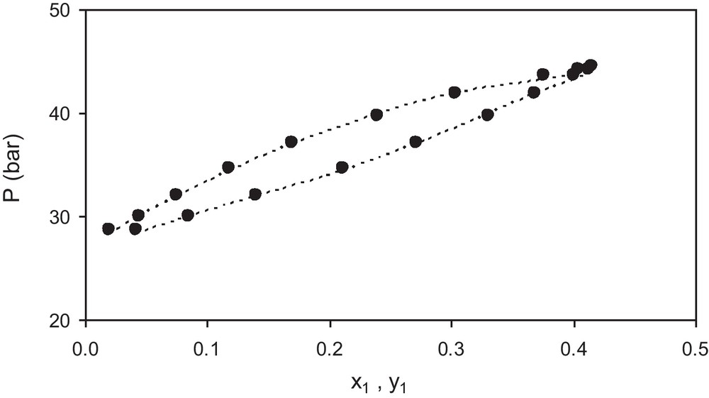
Experimental (●) and calculated values (-) of bubble pressure P -vs.- liquid mole fraction x1 and vapor mole fraction y1 for the system n-pentane (1) + 1-propanol (2) at T = 498 K. Experimental data are from Jung et al. [27].

Experimental (●) and calculated values (-) of bubble pressure P -vs.- liquid mole fraction x1 and vapor mole fraction y1 for the system n-butane (1) + methanol (2) at T = 443 K. Experimental data are from Courtial et al. [22].
5 Conclusions
Vapor-liquid equilibrium in mixtures alcohol + hydrocarbon at low and moderate pressures has been modeled using the EoS method (Peng-Robinson + Wong-Sandler + van Laar, PR/WS/VL) and appropriate comparison with other results from the literature using similar and more complex models have been done. The study and the results allow obtaining three main conclusions:
- • various factors must be considered when comparing results provided by different models;
- • the main factors are: the mathematical complexity of the model, the type and amount of basic properties and the number of adjustable parameters used by the model;
- • the equation of state method using appropriate mixing rules such as the one of Wong and Sandler can be used to model low and moderate pressure complex mixtures;
- • bubble pressures can be obtained with good accuracy with the PR/WS/VL model, giving absolute-average deviations below 5.3% for each isothermal data set and the overall absolute-average deviations is 1.7%;
- • the concentration in the vapor phase y1 can be obtained with good accuracy, giving absolute-average deviations bellow 9.3% for each isothermal data set and the overall absolute-average deviations and relative-average deviations are 2.3% and 0.08%, respectively.
Acknowledgments
The authors thank the Center for Technological Information of La Serena-Chile for computer support. CAF thanks the Direction of Research of the University of Concepción for the support through the research grant DIUC 211.011.054-1.0. JOV thanks the University of La Serena for especial support.
Vous devez vous connecter pour continuer.
S'authentifier