

Pressure
PcCritical pressure
TTemperature
TcCritical temperature
x1Solubility (component 1)
xcalCalculated solubility
xexpExperimental solubility
Greek symbols (super/subscripts)calCalculated
expExperimental
1 Introduction
Ammonia is a poisonous gas, harmful to people's health and is a severe environment contaminant. However, ammonia is necessary for some physiological and biological processes and is the raw material in petroleum refining and fertilizer manufacture. As an undesired material, the removal of ammonia from flue gases becomes an important issue since traditional ammonia–water absorption systems require additional rectification, increasing costs to prohibited limits [1]. Solvents that can absorb high quantities of ammonia and that do not need expensive additional separation processes represent an interesting alternative. Ionic liquids have shown to be that type of solvents and have received especial attention for process, such as synthesis, separations, catalysis, electrochemistry and waste gas separation [2–6]. Detailed information about various applications of ionic liquids is available in the literature [7–13]. The capture of ammonia by ionic liquids has also received some attention in the literature [1,12,13]. Experimental data show that solubility of ammonia in ionic liquids cover different ranges for different types of ionic liquids at the same temperature and pressure, and for several ionic liquids, solubility can be as high as 80% in mole fraction.
Different gas + ionic liquids mixtures have been studied in the literature using various thermodynamic models, mainly equations of state [16–20]. The application of an equation of state (EoS) to mixtures requires the use of mixing rules to represent the dependency of the EoS parameters on concentration and combination rules to represent the interaction between the unlike components in the mixture. The accuracy in correlating vapor–liquid equilibrium obtained by this method depends on the EoS used and the mixing and combining rule employed [21]. Also, binary interaction parameters must be introduced to obtain more accurate results. Such interaction parameters are obtained by fitting experimental phase equilibrium data at each temperature at which VLE is required. Considering also the difficulties of experimental measurements, besides the high cost in some cases, the development of alternative estimation methods, such as artificial neural networks have shown to be very successful for estimating VLE data that are of interest in chemical engineering [22–25].
For the specific case of ammonia + ionic liquids mixtures, some experimental studies at low and moderate pressures have been presented in the literature. Yokozeki and Shiflett [14,15] determined pressure–temperature–composition (P–T–x) solubilities of ammonia at room temperature ILs. The authors presented phase equilibrium data of four NH3 + IL mixtures: NH3 with [C4mim][BF4], [C4mim][PF6], [C6mim][C1] and [C2mim][Tf2N]. In another work, Yokozeki and Shiflett [15] reported P–T–x solubility of ammonia in [C2mim][Ac], [C2mim][SCN], [C2mim][EtOSO3] and [DMEA][Ac]. In both works, the authors observed high solubilities of ammonia in these ionic liquids. More recently, Li et al. [1] reported experimental solubilities of ammonia in four imidazolium-type ILs: [C2mim][BF4], [C4mim][BF4], [C6mim][BF4] and [C8mim][BF4]. The authors showed that all these ionic liquids have high solvency to capture NH3. To the best of the authors knowledge, specific applications, such as the one done in this work, in which P–T–x equilibrium data of ammonia + ionic liquids are correlated using artificial neural networks, have not been presented in the literature.
2 Application of artificial neural networks
Artificial neural networks are a computational model inspired in the behavior of natural neurons. A structure of neurons organized in different layers (known as architecture) receives data related to a given property, solubility for instance, and some independent variables that are supposedly related to the dependent main variable (temperature and pressure, for instance). The input and output variables are weighed by weights and shifted by a bias factor specific to each neuron. By optimization, the network learns the relation between the variables and stores the values of the weights and biases that give the lowest error between calculated and experimental data of the dependent variable (solubility in this work).
The artificial neural networks are “neural” in the sense that they have been inspired by neuroscience but not necessarily because they are faithful models of biological neural or cognitive phenomena. A neural network is characterized by:
- • its pattern of connections between the neurons (the architecture);
- • its method of determining the weights on the connections (training or learning process);
- • its activation function (relation between dependent and independent variables).
Good descriptions of ANN are given in the literature [26].
Taskinen and Yliruusi [27] presented a complete list of properties, mostly for organic substances, that have been analyzed in the literature, until 2003, using different approaches of ANN. Properties, such as normal boiling point, critical temperature, critical pressure, vapor pressure, heat capacity, enthalpy of sublimation, heat of vaporization, density, surface tension, viscosity, thermal conductivity, and acentric factor, among others, were thoroughly reviewed. Also, ANN has been previously used for gas solubility and phase equilibrium modelling in mixtures that do not include ionic liquids [28–32].
Applications of neural networks for the prediction of various thermodynamic properties of ionic liquids have been reported in a number of papers during the last ten years. Melting temperature have been studied by Carrera and Aires-de-Sousa [33], Bini et al. [34] and Torrecilla et al. [35], while other properties, such as density, viscosity and heat capacity have been modelled by Palomar et al. [36], Valderrama et al. [37,38] and Lashkarbolloki et al. [39,40]. Other authors have used ANN to model mixture properties, such as concentrations, infinite dilution activity coefficients [41–43]. Solubility modeling and Henry's law correlation using ANN have been done by Palomar et al. [36], Eslamimanesh et al. [25] and Safamirzaei and Modarres [44,45].
Table 1 shows selected papers on VLE calculation in binary mixtures of gas + ionic liquids using ANN. In the table, the type and number of systems studied, the number of data treated, the variable being correlated and predicted, the optimum architecture, and the type of information provided by the authors are clearly indicated. The symbol (*) in the last column indicates papers that provide the weight and bias matrixes, which correspond to the ANN model. As shown in the table, a drawback of most papers describing applications of ANN is that they do not give detailed information (data, architecture, activation functions, weight and bias matrix, or the program codes) to allow other researchers to reproduce the results and to make appropriate use of the ANN model. This is of special importance since it is known that a given ANN architecture cannot reproduce exactly the same results after each run of the network, unless the same weight and bias matrixes are used. In this paper, the authors provide as supplementary material the ANN model, consisting of the program codes to train the network and to predict the solubility of ammonia in IL, and also the files containing the data used for training and testing. All this will allow any reader to reproduce the results presented and to predict the solubility of ammonia in IL at other temperature for the systems studied. The codes can also be used to train the network with any other data if desired.
Selected papers on VLE calculations in binary mixtures using ANN. The symbol (*) in the last column indicates papers providing the weight and bias matrixes and NR means not reported.
| Reference | Type of mixtures | Number of systems | Number points | Number of independent variables | Dependent variable | layers optimum network | Provide data? | Provide ANN Program? |
| [42] | Organic solutes + ionic liquids | 64 | 916 | 8 | lnγ∞ | 3 | No | No |
| [25] | CO2 + ionic liquids | 24 | 1128 | 5 | 3 | Yes | No | |
| [43] | CO2 or CHF3 + ionic liquids | 9 | 1567 | 9 | lnγ∞ | 3 | Yes | No |
| [40] | Ethanol, water, acetonitrile, methanol, nitromethane + ionic liquids | 18 | 1571 | 4 | Cp | 3 | Yes | No |
| [44] | Gas + [C4mim] [PF6] | 7 | NR | 4 | KH | 3 | Yes | No* |
| [45] | Gas + [C4mim] [PF4] | 7 | 80 | 4 | xgas | 3 | Yes | No* |
| This work | NH3 + ionic liquids | 9 | 258 | 4 | 3 | Yes | Yes |
3 Solubility estimation using ANN
Nine binary ammonia + ionic liquids mixtures were considered for analysis and vapor–liquid equilibrium data of these systems were taken from the literature [1,14,15]. The nine ionic liquids are: [C4mim][BF4], [C4mim][PF6], [C2mim][BF4], [C6mim][BF4], [C8mim][BF4], [DMEA][AC], [C2mim][AC], [C2mim][Tf2N] and [C6mim][C1]. The training variables are the temperature and the pressure of the binary systems (T, P), being the target variable the solubility of ammonia in the ionic liquid. Then, to distinguish between the ionic liquids in the mixtures studied, two properties of the ionic liquids were used, the critical temperature and the critical pressure (Tc, Pc). Therefore, the number of input parameters for each case studied is equal to four (T, P, Tc, Pc). The output variable is equal to 1 (the solubility of ammonia in IL). Table 2 lists the pure component properties of all substances considered in this study. In the table, Tc is the critical temperature and Pc is the critical pressure. The values for the pure component properties were obtained from the literature [46,47].
Properties for all substances involved in this study.
| Components | Tc (K) | Pc (Mpa) | Reference |
| Ammonia | 405.5 | 11.35 | [46] |
| [C4mim][PF6] | 719.4 | 1.73 | [47] |
| [C2mim][BF4] | 596.2 | 2.36 | [47] |
| [C4mim][BF4] | 643.2 | 2.04 | [47] |
| [C6mim][BF4] | 690.0 | 1.79 | [47] |
| [C8mim][BF4] | 737.0 | 1.60 | [47] |
| [DMEA][AC] | 715.1 | 3.14 | [47] |
| [C2mim][AC] | 807.1 | 2.92 | [47] |
| [C2mim][Tf2N] | 1249.3 | 3.26 | [47] |
| [C6mim][C1] | 829.2 | 2.35 | [47] |
To develop an accurate ANN model for correlating and predicting the solubility of ammonia in ionic liquids in the form developed in this work, Matlab software was used and the following files were written:
- • an Excel file containing the independent variables: temperature, pressure and the two critical properties (Tc, Pc);
- • an Excel file containing the dependent variable, the solubility (x1);
- • a Matlab code that consists of two parts: a training section and a testing section.
In the training section, the program reads the input data (the two Excel files), defines the architecture, trains the defined network, generates the weight and bias matrixes, and stores such data for testing. In the testing section, the program reads the weight and bias matrixes, the Excel file containing the variables for which the solubility wants to be predicted and stores the results in an output file.
The most basic architecture normally used for this type of applications involves a back propagation feed-forward neural network containing three layers: the array input layer, one hidden layer and the output layer [24]. This type of network has proved to work well in another application for the estimation of physical and thermodynamic properties [22,24,37,38]. In the application described in this work, this simple architecture provides good results. Therefore, one hidden layer was required. Table 3 shows the source and range of the 208 data used for training of the artificial neural network.
Source and range of data used for training of the artificial neural network.
| Systems NH3 (1)+ | Reference | T (K) | N | Range of date | |
| Range of x1 | Range of P (MPa) | ||||
| [C4mim][PF6] | [14] | 283.4 | 4 | 0.371–0.862 | 0.138–0.517 |
| 298.0 | 5 | 0.351–0.854 | 0.174–0.796 | ||
| 298.6 | 5 | 0.344–0.853 | 0.184–0.822 | ||
| 347.2 | 5 | 0.253–0.791 | 0.345–2.385 | ||
| 355.8 | 5 | 0.239–0.773 | 0.371–2.700 | ||
| [C4mim][BF4] | [14] | 282.2 | 6 | 0.201–0.844 | 0.091–0.497 |
| 298.4 | 6 | 0.173–0.833 | 0.128–0.818 | ||
| 323.6 | 6 | 0.122–0.805 | 0.196–1.535 | ||
| 347.5 | 6 | 0.080–0.759 | 0.257–2.375 | ||
| 355.1 | 6 | 0.068–0.749 | 0.275–2.570 | ||
| [C2mim][BF4] | [1] | 293.0 | 5 | 0.2153–0.6921 | 0.140–0.550 |
| 298.0 | 5 | 0.1474–0.6176 | 0.110–0.550 | ||
| 323.0 | 5 | 0.0838–0.3896 | 0.120–0.630 | ||
| 333.0 | 5 | 0.1185–0.2549 | 0.200–0.570 | ||
| [C6mim][BF4] | [1] | 293.0 | 5 | 0.3815–0.7543 | 0.170–0.580 |
| 298.0 | 5 | 0.3673–0.6974 | 0.220–0.600 | ||
| 313.0 | 5 | 0.2722–0.6236 | 0.230–0.710 | ||
| 333.0 | 5 | 0.1280–0.5106 | 0.140–0.690 | ||
| [C8mim][BF4] | [14] | 293.0 | 5 | 0.4202–0.8081 | 0.130–0.540 |
| 298.0 | 5 | 0.2788–0.7476 | 0.120–0.610 | ||
| 323.0 | 5 | 0.1564–0.6002 | 0.100–0.59 | ||
| 333.0 | 5 | 0.1321–0.5022 | 0.120–0.59 | ||
| [DMEA][AC] | [15] | 283.2 | 6 | 0.477–0.865 | 0.136–0.491 |
| 298.1 | 6 | 0.475–0.864 | 0.163–0.769 | ||
| 348.0 | 6 | 0.454–0.853 | 0.433–2.689 | ||
| 372.8 | 4 | 0.675–0.844 | 1.994–4.249 | ||
| [C2mim][AC] | [15] | 282.5 | 6 | 0.624–0.877 | 0.321–0.550 |
| 298.2 | 6 | 0.601–0.871 | 0.463–0.896 | ||
| 324.5 | 6 | 0.538–0.852 | 0.792–1.774 | ||
| 348.5 | 6 | 0.473–0.819 | 1.098–2.891 | ||
| [C2mim][Tf2N] | [14] | 282.3 | 6 | 0.220–0.948 | 0.114–0.618 |
| 298.4 | 6 | 0.137–0.944 | 0.145–0.958 | ||
| 323.4 | 6 | 0.089–0.926 | 0.171–1.840 | ||
| 347.6 | 6 | 0.045–0.886 | 0.196–2.860 | ||
| [C6mim][C1] | [14] | 283.1 | 6 | 0.095–0.837 | 0.044–0.511 |
| 298.1 | 6 | 0.090–0.828 | 0.053–0.819 | ||
| 324.3 | 6 | 0.060–0.799 | 0.103–1.600 | ||
| 347.9 | 6 | 0.065–0.756 | 0.102–2.490 |
As an example, Table 4 shows the solubility.m Matlab code (provided as supplementary material) used for training and testing the solubility of ammonia. Once the ANN has been trained and the parameters of the network (weights and biases) are determined, they are stored in file w_solubility. It is expected that the values of x1 calculated by the network during training are close to the experimental values used for such training. In fact, the deviation between input values and correlated values is the objective function that must be minimized. Once this objective function has been minimized, it is assumed that the ANN learned the relation between the variables. How accurate was the learning is determined by the deviations between calculated and experimental values of solubility.
The Matlab code solubility.m used in this work to train the network.
| No. | % solubility.m |
| 1 | %************* |
| 2 | %This is the Matlab code for training an ANN with P–T data, using as independent variables |
| 3 | %the critical temperature, the critical pressure, the temperature and the pressure |
| 4 | % |
| 5 | %Reading independent variables for training (the critical temperature, the critical pressure, the temperature, |
| 6 | %and the pressure) |
| 7 | p = xlsread(’variables_for_training’);p = p’; |
| 8 | % %Reading the dependent variable for training (solubility); |
| 9 | t = xlsread(’solubility_for_training’);t = t’; |
| 10 | % Normalization of all data (values between –1 y +1) |
| 11 | [pn,minp,maxp,tn,mint,maxt] = premnmx(p,t); |
| 12 | % Definition of ANN:(topology, activation functions, training algorithm) |
| 13 | net = newff(minmax(pn),[5,4,1],{’tansig’,’tansig’,’purelin’},’trainlm’); |
| 14 | % Definition of frequency of visualization of errors during training |
| 15 | net.trainParam.show = 10; |
| 16 | % Definition of number of maximum iterations (epochs) and global error between iterations (goal) |
| 17 | net.trainParam.epochs = 500; net.trainParam.goal = 1e−4; |
| 18 | %Network starts: reference random weights and gains |
| 19 | w1 = net.IW{1,1}; w2 = net.LW{2,1}; w3 = net.LW{3,2}; |
| 20 | b1 = net.b{1}; b2 = net.b{2}; b3 = net.b{3}; |
| 21 | %First iteration with reference values and correlation coefficient |
| 22 | before_training = sim(net,pn); |
| 23 | corrbefore_training = corrcoef(before_training,tn); |
| 24 | %Training process and results |
| 25 | [net,tr] = train(net,pn,tn); |
| 26 | after_training = sim(net,pn); |
| 27 | % Back-Normalization of results, from values between -1 y +1 to real values |
| 28 | after_training = postmnmx(after_training,mint,maxt); after_training = after_training’; |
| 29 | Res = sim(net,pn); |
| 30 | % Saving results, correlated solubilities in an Excel file |
| 31 | dlmwrite(’solubility_correlated1.xls’,after_training,char(9)); |
| 32 | %Saving the nerwork (weigths and other files) |
| 33 | save w1_solubility |
| 34 | % |
| 35 | %solubility_prediction.m |
| 36 | %************** |
| 37 | % |
| 38 | %This is the Matlab code for predicting the solubility |
| 39 | % |
| 40 | %Reading weigth and other characteristics of the trained ANN saved in the file w1_solubility |
| 42 | load w1_solubility |
| 43 | % Reading of Excel file with new indepent variables to predict solubilities |
| 44 | pnew = xlsread(’variables_for_prediction’); pnew = pnew’; |
| 45 | % Normalization of all variable (values between –1 y +1) |
| 46 | pnewn = tramnmx(pnew,minp,maxp); |
| 47 | % Running the network and obtaining the predicted values of solubility. |
| 48 | anewn = sim(net,pnewn); |
| 49 | % Back-Normalization of results, from values between –1 and 1 to real values |
| 50 | anew = postmnmx(anewn,mint,maxt); anew = anew’; |
| 51 | % Saving results, predicted solubilities in an Excel file. |
| 52 | dlmwrite(’solubility_predicted1.xls’,anew,char(9)); |
Once the network is trained, three files are automatically created by the program solubility.m:
- • the file solubility_correlated.xls containing the values of the solubility of ammonia in the ionic liquid (x1) that the network learned during training;
- • the file w_solubility containing all matrixes that define the ANN model;
- • the solubility_predicted.xls containing the values of x1, determined by the trained network.
Matlab program (line 42 in Table 4) loads the ANN model stored in the file w_solubility, which contains the weight matrix defined during training. Then, the file variables_for_prediction.xls is automatically loaded. This file contains 50 rows with the values of the independent variables for those cases for which the solubility of ammonia in the ionic liquid has to be estimated. Using the model contained in the file w_solubility, the program determines the solubility for the 50 cases considered in this study for testing the ANN model. The program automatically creates an Excel file named solubility _predicted.xls where the predicted values for the solubility are stored.
It is well known that artificial neural networks are good tools for interpolation but not for extrapolation [26]. Therefore, the values of the independent variables (T, P) must be within the ranges used for training the network. In this study, the range of temperature was between 283 and 356 K, the range of P between 0.044 and 4.25 MPa and the range of x1 between 0.045 and 0.948, and the pure component properties of all substances considered are those listed in Table 2. Thus, if during testing any of the variables is outside the ranges used in training, good results are not guaranteed. In these cases, the ANN must be trained again, providing the necessary information in the file variables_for_training.xls and solubility_for_training.xls. The complete Matlab codes and the Excel files written for this work, with all the data used, are provided as supplementary material.
4 Results and discussion
Several network architectures were tested to select the most accurate and simple scheme. Since no additional information about the recommended number of layers and neurons has been found for the calculation of properties for any type of substances, the optimum number of layers and neurons was determined by trial and error. Simplicity of the architecture and accuracy of the results were the requirements imposed to find the optimum architecture. The accuracy of the chosen final network was checked by determining the relative and absolute deviations between the calculated values of x1 after training and data from the literature. The Fig. 1 shows the absolute percent deviation in correlating the solubility versus the number of layers in an architecture (10,N,1) and (5,N,1).
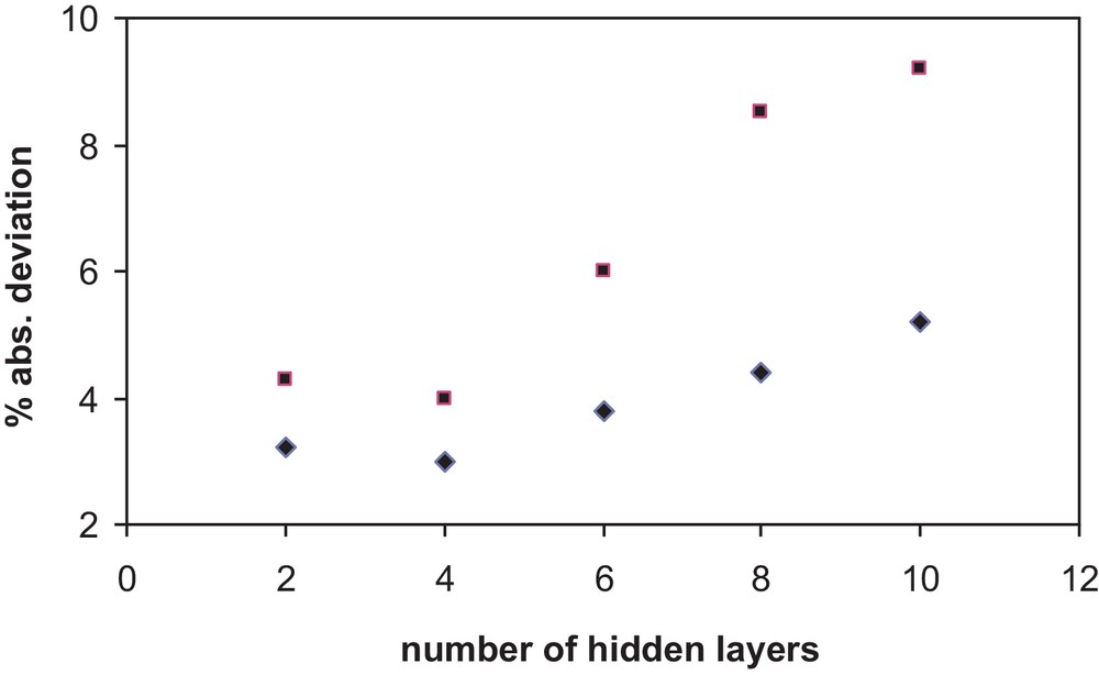
Absolute percent deviation in correlating the solubility versus the number of hidden layers N in an architecture (10,N,1) and (5,N,1).
The average absolute deviations , and relative deviations %Δx1, for a set of N data are defined as:
| (1) |
| (2) |
The final network used has five neurons in the input layer, one hidden layer of four neurons and one neuron in the output layer (5,4,1). This architecture has been chosen for the model proposed in this work.
During training, absolute individual deviations between correlated and literature values of solubility of ammonia in the ionic liquid were below 10% for most of the data points. The average absolute deviation was 3.3%, while average relative deviation was 0.31%. These values are considered to be accurate enough to state that the ANN learned in an appropriate way. Once the training was successfully done and the optimum network architecture was determined, 50 input data (Tc, Pc, T, P) of nine binary systems at other temperatures not used in the training process, included in the file variables_for_prediction.xls, were read by the program. The predicted 50 values of x1 calculated in the testing section of program are shown in Table 5.
Average deviations for the solubility of ammonia in ionic liquids, for nine complete isotherms not used during training. The last file shows the average absolute deviations for all the predicted points.
| Systems: NH3 (1) | T (K) | Pexp (MPa) | x1 exp | % x1 |
| [C4mim][PF6] | 324.0 | 0.274 | 0.292 | 0.5 |
| 0.423 | 0.389 | 1.8 | ||
| 0.583 | 0.492 | 1.9 | ||
| 1.083 | 0.681 | 0.7 | ||
| 1.567 | 0.828 | 2.2 | ||
| 1.4 | ||||
| [C4mim][BF4] | 298.6 | 0.127 | 0.174 | 4.2 |
| 0.196 | 0.267 | 2.5 | ||
| 0.271 | 0.367 | 2.5 | ||
| 0.437 | 0.548 | 0.3 | ||
| 0.616 | 0.683 | 2.9 | ||
| 0.807 | 0.834 | 0.9 | ||
| 2.2 | ||||
| [C2mim][BF4] | 313.0 | 0.140 | 0.126 | 4.4 |
| 0.290 | 0.255 | 2.3 | ||
| 0.370 | 0.324 | 4.9 | ||
| 0.530 | 0.447 | 6.5 | ||
| 0.620 | 0.526 | 9.6 | ||
| 5.5 | ||||
| [C6mim][BF4] | 323.0 | 0.180 | 0.1898 | 2.0 |
| 0.390 | 0.3548 | 4.7 | ||
| 0.460 | 0.4106 | 1.1 | ||
| 0.540 | 0.4550 | 0.8 | ||
| 0.710 | 0.5779 | 7.4 | ||
| 3.2 | ||||
| [C8mim][BF4] | 313.0 | 0.180 | 0.283 | 6.7 |
| 0.300 | 0.398 | 9.3 | ||
| 0.390 | 0.505 | 1.7 | ||
| 0.500 | 0.574 | 3.1 | ||
| 0.600 | 0.644 | 1.1 | ||
| 4.4 | ||||
| [DMEA][AC] | 322.7 | 0.277 | 0.466 | 1.4 |
| 0.463 | 0.609 | 0.6 | ||
| 0.786 | 0.704 | 3.4 | ||
| 0.980 | 0.757 | 2.0 | ||
| 1.250 | 0.809 | 1.2 | ||
| 1.521 | 0.860 | 0.6 | ||
| 1.5 | ||||
| [C2mim][AC] | 298.3 | 0.470 | 0.599 | 0.3 |
| 0.667 | 0.730 | 0.8 | ||
| 0.765 | 0.788 | 0.6 | ||
| 0.820 | 0.825 | 0.3 | ||
| 0.850 | 0.839 | 0.1 | ||
| 0.898 | 0.871 | 0.9 | ||
| 0.5 | ||||
| [C2mim][Tf2N] | 299.4 | 0.136 | 0.171 | 17.1 |
| 0.287 | 0.430 | 8.3 | ||
| 0.434 | 0.568 | 0.6 | ||
| 0.698 | 0.768 | 0.6 | ||
| 0.969 | 0.921 | 0.1 | ||
| 0.994 | 0.943 | 0.9 | ||
| 4.6 | ||||
| [C6mim][C1] | 297.8 | 0.059 | 0.086 | 13.8 |
| 0.133 | 0.231 | 0.3 | ||
| 0.216 | 0.337 | 7.0 | ||
| 0.377 | 0.537 | 2.2 | ||
| 0.647 | 0.728 | 2.1 | ||
| 0.816 | 0.828 | 0.3 | ||
| 4.3 |
Table 5 shows the individual absolute deviations for the solubility of ammonia in the ionic liquid x1, predicted by the proposed ANN model for nine isotherms not used during training. The last file in the table shows the average absolute deviations for all the predicted points. As seen in Table 5, the ANN model reproduces the solubility of ammonia in the ionic liquid x1 with average absolute deviations from 0.5% to 5.5% for each isothermal data set. The average relative deviations vary between –4.4% and 4.4% for each isothermal data set. The maximum individual absolute deviation in x1 is 17.1%.
Fig. 2 shows experimental and calculated values of solubility of ammonia in the ionic liquid (x1) vs pressure (P) for the system NH3 (1) + [C4mim][BF4] (2) at T = 298.6 K, while Fig. 3 shows the same for the mixture NH3 (1) + [C8mim][BF4] (2) at T = 313 K. In these figures, symbol (•) represents the experimental data and the dashed line (---) represents the calculated values. As seen in the figures, both cases show the good agreement found between ANN model estimates and experimental data.
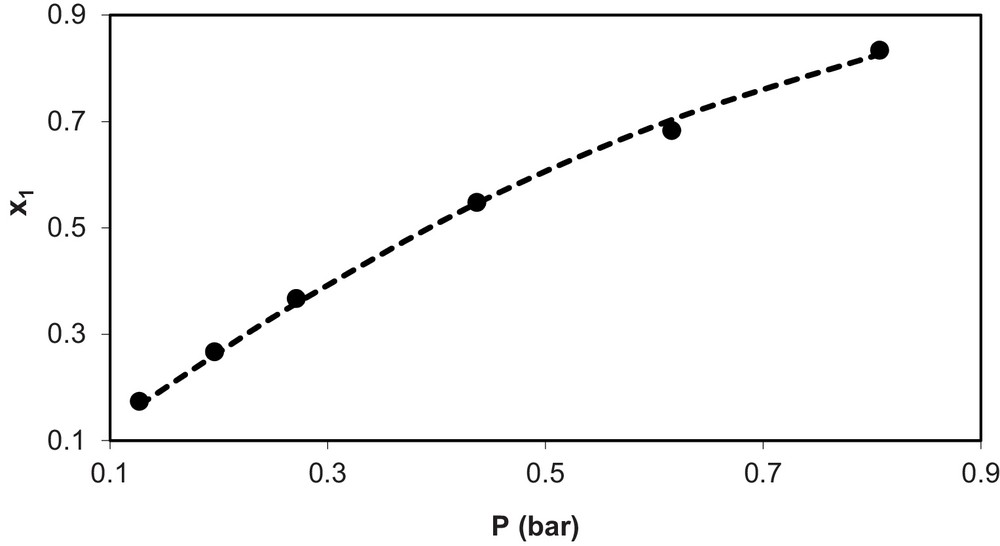
Experimental (•) and calculated values (--) of solubility of NH3 (x1) vs. pressure (P) for the system NH3(1) + (C4MIN)(BF4) (2) at T = 298.6 K.
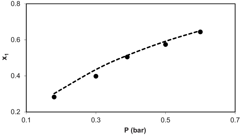
Experimental (•) and calculated values (--) of solubility of NH3 (x1) vs. pressure (P) for the system NH3(1) + (C8MIN)(BF4) (2) at T = 313 K.
Some final words about the meaning of the good results obtained for the estimated solubility are necessary to highlight the importance of accurately predicting this variable. Of the systems treated in this paper, the system NH3 + [C2mim][AC] presents high solubility (> 0.5 in mole fraction) in a wide range of temperature (282 to 348 K) while for systems, such as NH3 + [C6mim][C1] in similar ranges of temperature, solubility is lower than 0.1 in mole fraction. The proposed ANN model was able to correlate and predict the solubility with low deviations for most cases. In the correlation, some few points showed deviations higher than 10% and in the prediction, only two of the fifty predicted points showed deviations higher than 10%. In these cases, the highest deviations obtained are associated with the quality of the experimental data. As Yokozeki and Shiflett [14] wrote: “rather large uncertainties in low x1 values are due to the inaccuracy in weight measurements of very small amounts of NH3”.
In summary, this paper shows that ANN represent a good tool for correlating and predicting solubility of ammonia in ionic liquids at temperatures for which no experimental data exist. The next natural step in this type of studies would be predicting the solubility of ammonia in other ionic liquids not used for obtaining the ANN model. To do this, however, much more data would be needed, which are not available at this time.
5 Conclusions
An artificial neural network model has been used to correlate and predict the solubility of ammonia in ionic liquids for nine binary ammonia + ionic liquid systems. The study and the results allow obtaining two main conclusions:
- • the solubility of ammonia in ionic liquid, x1, can be obtained with good accuracy, giving absolute average deviations below 5.6%, for each isothermal data set and overall absolute average deviations of 3.0%;
- • only in the range of low solubilities (below 0.2 in mole fraction) did the predicted solubilities give deviations higher than 10%.
Acknowledgements
The authors thank the support of the Chilean National Council for Scientific and Technological Research (CONICYT) through the research grant FONDECYT 1070025. JOV thanks the Direction of Research of the University of La Serena-Chile and the Center for Technological Information of La Serena-Chile for permanent support. CAF and FQ thank the Direction of Research of the University of Concepcion-Chile for the support through the research grant DIUC 211.011.054–1.0.