Elastic models, lattice dynamics and finite size effects in molecular spin crossover systems

Cristian Enachescu; William Nicolazzi

doi:10.1016/j.crci.2018.02.004

Account/Revue

Elastic models, lattice dynamics and finite size effects in molecular spin crossover systems

Cristian Enachescu ¹ ; William Nicolazzi ²

¹ Faculty of Physics, Alexandru Ioan Cuza University of Iasi, Iasi 700506, Romania
² Laboratoire de chimie de coordination, CNRS UPR 8241 and Université de Toulouse, UPS, INP, France

Comptes Rendus. Chimie, Volume 21 (2018) no. 12, pp. 1179-1195.

Résumé

The experimental studies of spin-crossover compounds switched in the last decade from bulk measurements and macroscopic observations to the nanoscale and microscopic approaches. In this context, new and sometimes unexpected behaviours have been documented, which could be partially described only by the classical phenomenological models developed in the last period of the last century. In this context, the development of more complex models, able to reproduce the nucleation and domain propagation within the material, has proved to be not a whim of some theoreticians but a necessity, which facilitated the full understanding of observed phenomena and even made premises for further experiments. Here, we present and analyse various elastic models identifying their common points and differences and discuss how they can be used for the study of microscopic phenomena as the cluster formation, stability and propagation or for the study of finite size effects in spin-crossover nanoparticles, with open boundary conditions or embedded in various matrices.

Métadonnées

Reçu le : 2017-11-18
Accepté le : 2018-02-12
Publié le : 2018-03-24

DOI : 10.1016/j.crci.2018.02.004

Mots clés : Spin crossover, Elastic models, Finite size effects, Monte Carlo simulations, Lattice dynamics

Affiliations des auteurs :

Cristian Enachescu ¹ ; William Nicolazzi ²

¹ Faculty of Physics, Alexandru Ioan Cuza University of Iasi, Iasi 700506, Romania
² Laboratoire de chimie de coordination, CNRS UPR 8241 and Université de Toulouse, UPS, INP, France

@article{CRCHIM_2018__21_12_1179_0,
     author = {Cristian Enachescu and William Nicolazzi},
     title = {Elastic models, lattice dynamics and finite size effects in molecular spin crossover systems},
     journal = {Comptes Rendus. Chimie},
     pages = {1179--1195},
     publisher = {Elsevier},
     volume = {21},
     number = {12},
     year = {2018},
     doi = {10.1016/j.crci.2018.02.004},
     language = {en},
}

TY  - JOUR
AU  - Cristian Enachescu
AU  - William Nicolazzi
TI  - Elastic models, lattice dynamics and finite size effects in molecular spin crossover systems
JO  - Comptes Rendus. Chimie
PY  - 2018
SP  - 1179
EP  - 1195
VL  - 21
IS  - 12
PB  - Elsevier
DO  - 10.1016/j.crci.2018.02.004
LA  - en
ID  - CRCHIM_2018__21_12_1179_0
ER  -

%0 Journal Article
%A Cristian Enachescu
%A William Nicolazzi
%T Elastic models, lattice dynamics and finite size effects in molecular spin crossover systems
%J Comptes Rendus. Chimie
%D 2018
%P 1179-1195
%V 21
%N 12
%I Elsevier
%R 10.1016/j.crci.2018.02.004
%G en
%F CRCHIM_2018__21_12_1179_0

Cristian Enachescu; William Nicolazzi. Elastic models, lattice dynamics and finite size effects in molecular spin crossover systems. Comptes Rendus. Chimie, Volume 21 (2018) no. 12, pp. 1179-1195. doi : 10.1016/j.crci.2018.02.004. https://comptes-rendus.academie-sciences.fr/chimie/articles/10.1016/j.crci.2018.02.004/

Version originale du texte intégral

1 Introduction

Spin-crossover (SCO) compounds are transition metal complexes in thermodynamic competition between the low-spin (LS) state, stable at low temperature, and the high-spin (HS) state, stable at higher temperature. These states have not only different magnetic, optical and vibrational properties but also different molecular volumes, with a slightly larger volume for the HS state. The change in volume during the transition results in the building-up of stress in the crystal and therefore is at the origin of elastic interactions and more generally at the origin of all elastic collective behaviours called cooperativity, which, if strong enough, are responsible at the macroscopic scale for the first-order transition accompanied by bistability and hysteresis phenomena. At the microscopic scale, elastic interactions induce nucleation, cluster formation and growth of like-spin domains, that is, domains of adjacent molecules in the same spin state.

The simplest approaches for the study of the macroscopic behaviour of SCO compounds are mean-field models, which imply random distribution of HS and LS molecules during the transition. Mean-field models have successfully reproduced a number of experimental curves (thermal transition, relaxations, and photoexcitation), mainly in the case of less cooperative diluted SCO compounds. These models, which remain widely used, represent a valuable tool in SCO research. However, these models do not include short-range interactions and therefore do not allow an appropriate analysis of the propagation of molecular switching inside the sample. For a deeper microscopic description of nucleation and domain growth processes, different models should be used. One of the simplest models introducing short-range interactions is the Ising model, adapted for the study of SCO compounds by replacing the classical magnetic field with a temperature-dependent field. The Ising model, reviewed in the article of Pavlik and Linares in this special issue, has been used to successfully treat both the dynamic and static properties [1,2] of SCO compounds in the framework of Metropolis or Arrhenius approaches with only short-range interactions or a combination of short-range and long-range interactions. Although Ising-like models can reproduce to some extent both macroscopic and microscopic behaviours, they describe only partially the relations between elastic interactions and cooperativity due to a lack of a simultaneous treatment of local distortions and global deformations. Indeed, the interactions between neighbouring sites are fixed and the lattice cannot be deformed. More complex models aiming to improve this deficiency have been developed. A first model based on the ligand field theory discussing the effect of coupling between d-electrons and lattice strains has been proposed by Kambara [3], following the phenomenological description of Slichter and Drickamer [4]. In his lattice expansion model using the Eshelby defect theory based on continuum medium mechanics considerations [5], Spiering et al. [6] emphasized that elastic interactions arise from stresses because of changes in the volume, shape and elasticity of the lattice during the transition, but still treated the system in a mean-field approach. In addition, Kambara was the first to introduce intramolecular distortions as a dynamic variable and considered the intermolecular coupling in his model [7]. Meanwhile, Zimmermann and Konig [8] took into account the spin–orbit coupling and the effect of low-symmetry ligand fields and considered the volume expansion of the elastic medium, which would induce an additional contribution to the lattice energy. A decade later, it was stated that the interaction constant can be explained by the elasticity theory in a proportion of around 80% [9]. These “realistic” models, despites their huge interest, have not been extensively used by the SCO community for the complexity of calculations and the large number (mostly unknown) material parameters.

An intermediate model between the Ising-like model and elastic defect theory is the atom–phonon coupling model [10,11], in which the SCO compounds are modelled in a similar way as in the Ising-like model, but neighbouring molecules are linked by springs, whose elastic constant can take three different values according to the spin states of the closest molecules (HS–HS, HS–LS or LS–LS).

New experimental results in the last decade called for the development of more advanced and sophisticated models. After years of theoretical suppositions and partial experimental proofs [12–14], a first direct answer to the fundamental question, “does the heterogeneous phase separation exist and does it play a role in the spin crossover phenomena?” [15], has been provided by Pillet et al. [16] by diffraction analysis of high-quality single crystals, constituting an indubitable proof of the existence of a spin-like domain formation. In a pioneering work, Bonnet et al. [17], followed by several articles of Versailles group [18,19] and Toulouse group [20,21] (for an overview see also Ref. [22]), have visualized the phase separation in a single crystal using optical microscopy. The various optical microscopy results showed that the process always starts from a corner of the crystal, and the dependence of the evolution of subsequent clusters on the size, shape and thermal history of the crystal has been carefully analysed. Further experimental works have investigated the velocity of propagation of the interface between the two phases [23,24]. The role of lattice mismatches (elastic stress and strain) [24] and latent heat in this process was also demonstrated [25]. Other recent experiments showing the building-up of an elastic step after photoexcitation using a femtosecond laser have also been explained in terms of the propagation of elastic distortions [26].

To correctly describe the microscopic mechanism of SCO phenomena and to reproduce the new experimental results, the logical development of models implied the replacement of ambiguous short- and long-range interactions with genuine elastic interactions arising from lattice distortions because of the molecular size difference between the LS and HS states. This led to a new class of models—so-called “ball and spring models”, which consider the molecules as rigid and usually unfixed spheres linked by springs that can be compressed or elongated during the transition resulting in practically an infinite number of possible interaction terms between molecules. In the pioneering years, at the end of the first decade of the new millennium, different ball and spring models have been independently and almost simultaneously proposed by a few groups of researchers working in the SCO field [27–33]. Even if all these models are based on the same idea, formal differences can be detected in the form of Hamiltonians used in the theoretical approaches, in the internal structure and shape of the samples, as well as in the methods used in the simulations. The subsequent period has been devoted to applications and development of models for reproducing various experimental behaviours of SCO compounds, including new emerging phenomena observed in the case of micro- and nanoparticles. The present review is organized as follows: first, we present the most important ball and spring models, emphasizing on the similarities and differences in between. Then we discuss their applications with the accent on size reduction effects.

2 A journey to various types of elastic models

2.1 Hamiltonians

The starting point for all elastic Hamiltonians is the simple Ising-like Hamiltonian [1,34], which is discussed in more details in the review of Pavlik and Linares [35]. By associating a fictitious spin with each molecule ( $S_{i} = \pm 1$ for HS (LS) state), the short-range interactions $J$ and long-range interactions $G$ can be written as exchange interactions in the Hamiltonian:

H = \frac{1}{2} \sum_{i} (D - k_{B} T \ln g) S_{i} - J \sum_{i, j} S_{i} S_{j} - G \sum_{i} S_{i} 〈 S 〉

(1)

where

D

and g are the energy difference and the degeneracy ratio between the two states,

k_{B}

is the Boltzmann constant and

T

is the temperature. The HS fraction can be expressed as a function of the “fictitious magnetization”

〈 S 〉

n_{HS} = \frac{1 + 〈 S 〉}{2}

(2)

In the elastic models, the interaction terms are replaced in the Hamiltonian with an intermolecular elastic potential [27,31–33,36–48]:

H = \frac{1}{2} \sum_{i} (D - k_{B} T \ln g) S_{i} + \sum_{〈 i, j 〉} V_{i j}^{inter}

(3)

The most general expression of the elastic potential can be written as

\sum_{〈 i, j 〉} V_{i j}^{inter} = \sum_{i, j} \frac{k}{2} δ x_{i j}^{2}

(4)

where

k

stands for the bond stiffness parameter (which is the simple elastic constant

k

in the case of a harmonic potential) and

δ x_{i j}

corresponds to the individual spring elongations between all neighbouring molecules in the system. The elastic constant, standing for both short- and long-range interaction constants in the Ising-like models, is the key parameter in the model accounting for the cooperativity. Although most of articles on the elastic models used arbitrary values for this constant, it was recently shown that its value can be directly related to the bulk modulus

B

, which can be experimentally determined [9]. The relation between the two parameters can be expressed as

k = 3 c_{0} B

[46,49], where

c_{0}

is the unit cell length, which for standard values of

c_{0} = 10^{- 9} m

and

B = 50 kbar

[9] results in a value for

k

of around 5 N/m for a cubic system. This value for the elastic constant has been confirmed by an approach based on the ligand field theory [46].

In the case of a hexagonal lattice [31], all neighbours are equivalent and the individual spring elongations can be written as

δ x_{i j} = d_{i j} - (l_{0 i j} + r_{i} + r_{j})

(5)

where

d_{i j}

are the distances between the centres of

i th

and

j th

sites,

r_{i}

and

r_{j}

are the radii of

i

and

j

molecules,

l_{0 i j}

is the natural bond length of the springs, and therefore the elastic potential can be written as

\sum_{〈 i, j 〉} V_{i j}^{inter} = \sum_{i, j} \frac{k}{2} {[d_{i j} - (l_{0 i j} + r_{i} + r_{j})]}^{2}

(6)

Expression (6) was mainly used in the so-called mechanoelastic model, first mentioned in Ref. [31].

In the case of a rectangular lattice, to maintain the topology of the bond network and to ensure the mechanical stability with respect to the shear distortions, the presence of second neighbour interactions is needed and consequently the potential will be written as

\sum_{〈 i, j 〉} V_{i j}^{inter} = \sum_{i, j} \frac{k_{1}}{2} {[d_{i j} - (l_{0 i j} + r_{i} + r_{j})]}^{2} + \sum_{i, k} \frac{k_{2}}{2} {[d_{i k} - (l_{0 i k} + r_{i} + r_{k})]}^{2}

(7)

where

〈 i, j 〉

and

〈 i, k 〉

denote, respectively, the first and the second neighbour bonds.

Simple geometrical considerations give the following relation between $l_{0 i j}$ and $l_{0 i k}$ (see Fig. 1):

l_{0 i k} = \sqrt{2} l_{0 i j} + (\sqrt{2} - 1) (r_{i} + r_{k})

(8)

Fig. 1
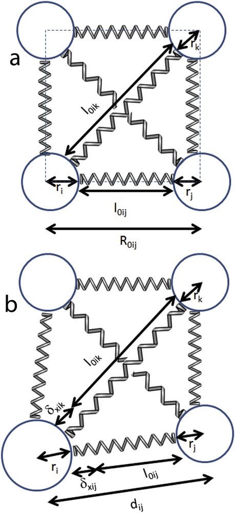
Schematic illustration of the elastic model for a system in the initial configuration with all molecules identical (a) and during the transition with the presence of a larger molecule (b).

A first approach of the interaction potential assumed the closest molecular spheres in contact at equilibrium and therefore $l_{0 i j} = 0$ . In this case, taking into account relation (8), the elastic potential will be written in the following form:

\sum_{〈 i, j 〉} V_{i j}^{inter} = \frac{k_{1}}{2} {\sum_{i, j} [d_{i j} - (r_{i} + r_{j})]}^{2} + \frac{k_{2}}{2} \sum_{i, k} {[d_{i k} - \sqrt{2} (r_{i} + r_{k})]}^{2}

(9)

This expression of the elastic potential has been used in the original elastic models in SCO compounds [27,28,37,38] (the one-dimensional [1D] case has been proposed in 2001 by J. Nasser in a study [50] who now can be interpreted as a precursor of the current elastic models).

An alternative approach to keep the rectangular structure during simulations without using the second-order neighbour interactions was more recently proposed in the so-called “stretching and bending model” [49]. It considers an angular harmonic potential corresponding to the angle $θ$ between two pairs of molecules sharing the same vortex (see Fig. 1). In this case, the second term of potential (7) is replaced with a bending oscillator:

\sum_{〈 i, j, k 〉} V_{i j k} = \sum_{i, j, k} \frac{k_{2}}{2} {[θ_{i j k} - θ_{0}]}^{2}

Another expression for the intermolecular potential $V_{i j}^{inter}$ implies the use of exponential functions for nearest neighbours in the following form:

\sum_{〈 i, j 〉} V_{i j}^{inter} = \sum_{i, j} C [\exp (α (δ x_{i j} - u_{0})) + \exp (- β (δ x_{i j} - u_{0}))]

where

C

α

β

and

u_{0}

are constants and

u_{0}

is chosen such as the sum of exponentials in the above equation has its minimum at

δ x_{i j} = 0

Considering the equilibrium distances between the mass centres of $〈 i, j 〉$ molecules

R_{0 i j} = l_{0 i j} + r_{i} + r_{j} and R_{0 i k} = l_{0 i k} + r_{i} + r_{j}

(10)

the elastic potential can be written as

\sum_{〈 i, j 〉} V_{i j}^{inter} = \frac{k_{1}}{2} \sum_{i, j} {(d_{i j} - R_{0 i j})}^{2} + \frac{k_{2}}{2} \sum_{i, k} {(d_{i k} - R_{0 i k})}^{2}

(11)

Then, the total Hamiltonian can be expressed in terms of an Ising-like Hamiltonian (1) as

H = \sum_{i} (\frac{1}{2} (D - k_{B} T \ln g) - k ρ_{1} \sum_{j = 1}^{z} (d_{i j} - ρ_{0})) S_{i} + k ρ_{1}^{2} \sum_{〈 i, j 〉} S_{i} S_{j} + \frac{k}{2} \sum_{〈 i, j 〉} {(d_{i j} - ρ_{0})}^{2} + 2 k N ρ_{1}^{2}

(12)

where

ρ_{0} = l_{0 i j} + r_{H} + r_{L}

and

ρ_{1} = r_{H} - r_{L}

This Hamiltonian in the above form is the basis of the so-called electroelastic approach for SCO complexes [40–42].

In the case of the so-called anharmonic model, the values of $k_{1}$ and $k_{2}$ depend on the equilibrium intermolecular distances (as the bulk modulus in experimental data) and can be expressed in the following form:

k_{1} = k_{01} + k_{11} {[d_{i j} - (l_{0 i j} + 2 r_{HS})]}^{2}

(13)

k_{2} (d_{i k}) = k_{02} + k_{12} {[d_{i k} - \sqrt{2} (l_{0 i k} + 2 r_{HS})]}^{2}

(14)

The anharmonicity has been introduced by considering the Lennard-Jones intermolecular interaction potential whose equilibrium distances and minimum energies at zero temperature can be dependent on the spin state of the molecules forming the bonds [32]. This model allows a better control of thermal expansion phenomena, which is known to be different in the two molecular phases, due to different elastic and vibrational properties. The so-called two-variable anharmonic model has been used for the simulation of X-ray diffraction experiments, reproducing the crystallographic phase separation (Bragg peak splitting) observed during the thermal spin transition or during nonequilibrium phase transformation kinetics like photoexcitations or thermal quenching process [33]. In a similar way as the electroelastic model, the anharmonic model has been rewritten as an Ising-like model [48]:

H = \sum_{〈 i, j 〉} [J (d_{ij}) S_{i} S_{j} + h (d_{ij}, T) (S_{i} + S_{j}) + D (d_{ij})]

(15)

where

D (d_{ij})

is the mean lattice cohesion energy. The lattice degrees of freedom and the fictitious Ising spins are coupled through the exchange-like terms J(d_ij)S_iS_j and h(d_ij)(S_i + S_j). These three quantities can be expressed as a function of the Lennard-Jones interaction potentials of the three possible bonds

A_{i j} V_{i j}^{inter}

with ij = HH, LL, HL (or LH) (Fig. 2):

J (d_{ij}) = \frac{A_{HH} V_{HH}^{inter} + A_{LL} V_{LL}^{inter} - 2 A_{HL} V_{HL}^{inter}}{4}

(16)

h (d_{ij}) = \frac{A_{HH} V_{HH}^{inter} - A_{LL} V_{LL}^{inter}}{4} + \frac{D - k_{B} T ln (g)}{4}

(17)

D (d_{ij}) = \frac{A_{HH} V_{HH}^{inter} + A_{LL} V_{LL}^{inter} + 2 A_{HL} V_{HL}^{inter}}{4}

(18)

Fig. 2
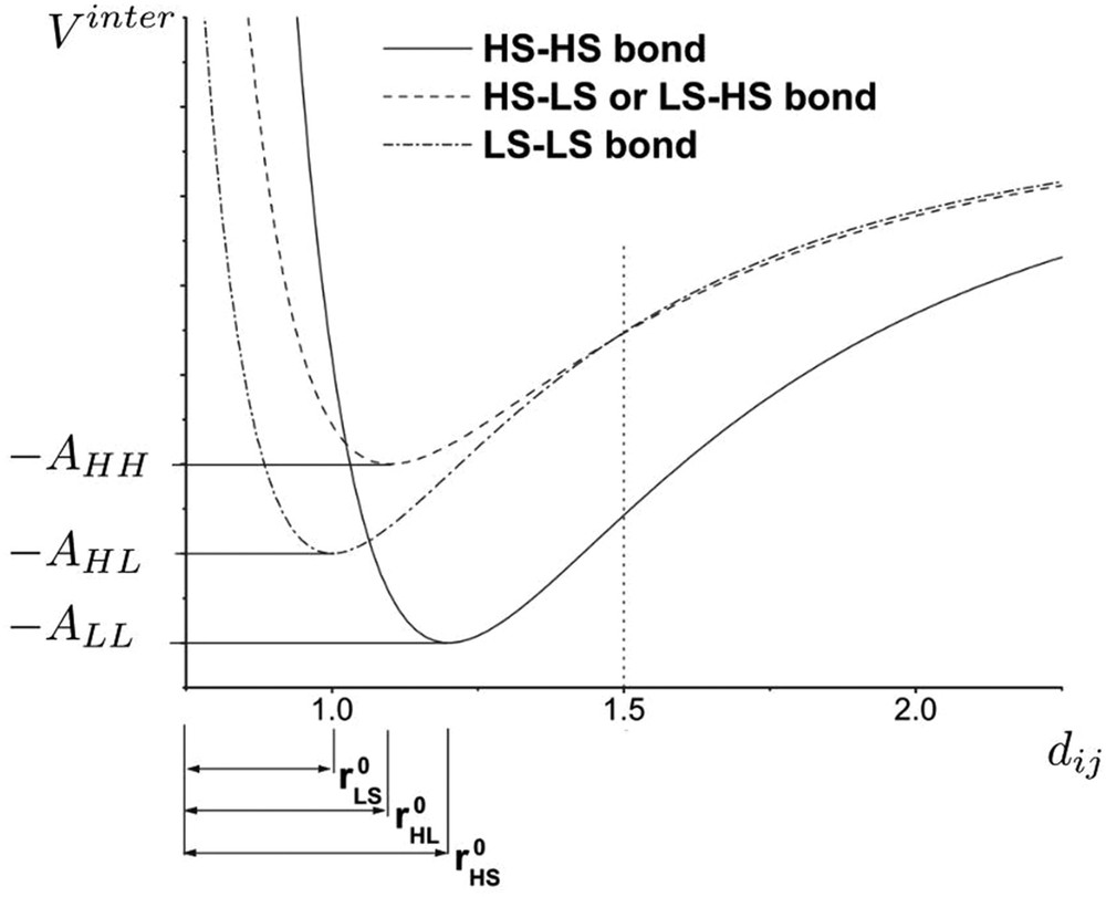
Spin-state-dependent Lennard-Jones potential for the anharmonic spin–phonon model. Equilibrium intersite distances and cohesion energies are dependent on the spin state of the two nearest-neighbour molecules (modelled by Ising fictitious spins) forming the bond.

A second-order Taylor development of the three Lennard-Jones potentials around the equilibrium intersite spacings permits to retrieve a Hamiltonian with a similar form to Eq. (12). When the minimum energies of the Lennard-Jones potentials are spin state dependent, the zero-order term corresponds to a lattice-independent Ising coupling. A main consequence is the presence of a clustering process during the spin state change in a system with periodic boundary conditions [48].

As a final note on models, let us mention two other possible terms, which have been considered in some cases. In addition to the intermolecular potential (9), an intramolecular adiabatic potential has also been considered [27], which can be written in the framework of the parabolic approximation for LS and HS molecules as follows:

V^{intra} (x) = \frac{A}{2} (d + b {(c - x)}^{2} + a x^{2} - \sqrt{4 J^{2} + {(d + b {(c - x)}^{2} - a x^{2})}^{2}})

(19)

where a, b, c and d are constants and x is the difference between the radius of the molecule and the LS molecular radius.

When elastic models are investigated by molecular dynamics methods, a kinetic term has also to be added, with the following expression:

K = \sum_{i = 1}^{N} \frac{p_{i}^{2}}{2 m} + \sum_{i = 1}^{N} \frac{P_{i}^{2}}{2 M}

(20)

where

P_{i}

and p_i represent the conjugate momenta of the coordinate of the centre

x_{i}

and of the radius

r_{i}

, respectively, for the

i' th

molecule. M and m correspond to the molecular and ligand masses, respectively. The molecular dynamics is often used together with an exponential-type potential; however, it was stated that the use of harmonic or Lennard-Jones potentials does not change the qualitative results of the elastic models.

2.2 Simulation procedures

The simulations using elastic approaches imply two different processes: the switch of spins and the change in molecular positions. These two processes can be separated (first one decides if a molecular switch is accepted or rejected and afterwards, if the spin changes, the new positions of molecules are found) or coupled (the decision of acceptance or rejection is taken after both the switch and the new molecular positions are determined).

During the first process, (1) one attributes to the molecule a spin state, taking into account the degeneracy ratios $g_{LS} / (g_{LS} + g_{HS})$ or $g_{HS} / (g_{LS} + g_{HS}) /$ , (2) the spin change is accepted or rejected using the Metropolis criterion (vide infra) or (3) it is also possible to consider that the spin changes with a probability depending on the local pressure.

The use of the Monte Carlo Metropolis standard procedure has following the steps: (1) one calculates the energy of the system in its actual state, according to the chosen Hamiltonian; (2) after considering one molecular switch (and finding or not the new molecular positions, depending on the model), one computes the new energy of the system; (3) one calculates the Metropolis probability

P = \min (1, \exp (- \frac{(D - k_{B} T \ln g) S_{i}^{final} + (V_{elastic}^{final} - V_{elastic}^{initial})}{k_{B} T}))

(21)

and then generates a random number

r \in (0,1)

. If

r \leq P

the switching is accepted; otherwise, the switching is not accepted. In this last case, all the molecules return to the positions before point (2). A Monte Carlo step is concluded when all the molecules in the system have been checked once on average.

As the Metropolis procedure is less suitable for the study of the HS–LS relaxation or for other nonequilibrium phenomena, in Refs. [26,31,51,52], the molecular spin switching is decided through a kinetic Monte Carlo algorithm, taking into account the transition rates that depend on the energy barrier between the states rather than on the energy difference between the states. The following HS → LS and LS → HS switching probabilities have been defined based on the Monte Carlo Arrhenius-type dynamics and considering the local pressure influence on every molecule:

P_{HS \to LS}^{i} = \frac{1}{τ} \exp (\frac{D - k_{B} T \ln g}{2 k_{B} T}) \exp (- \frac{E - κ p_{i}}{k_{B} T})

(22)

P_{LS \to HS}^{i} = \frac{1}{τ} \exp (- \frac{D - k_{B} T \ln g}{2 k_{B} T}) \exp (- \frac{E + κ p_{i}}{k_{B} T})

(23)

respectively. Here

τ

is a scaling constant, chosen so that the above probabilities are well below unity at any temperature, κ is a scaling factor between the local pressure and the activation energy of the individual molecule, whereas

E

corresponds to the activation energy of the HS → LS relaxation relative to a global reference state in which all of the molecules are in the HS state.

p_{i}

is the local pressure acting on molecule

i

, defined as

p_{i} = \sum_{neighbours springs} (k / A) δ x_{i j}

, where

k

is the spring constant, A the molecular cross-sectional area and

\sum_{neighbours springs} δ x_{i j}

is the algebraic sum at mechanical equilibrium of elongations of neighbouring springs (here taken positive for elongated springs and negative for compressed ones).

The new molecular positions in the system are found by (1) relaxing mechanically the lattice, considering small displacements on all axes for randomly selected molecules, (2) considering the equations of motion in the framework of Nosé–Hoover formalism or (3) deterministically calculating the motion of molecules, by solving exactly a system of differential equations.

The Nosé–Hoover formalism [27] implies the following equations of motion, with the Hamiltonian of the thermal reservoir given by $H_{therm} = (P_{S}^{2} / 2 Q) + 3 N k_{B} T \ln s$ ( $s$ is a scaling factor, $P_{S}$ is the conjugated momentum of $s$ and $Q$ is the effective mass), which are then added to the chosen Hamiltonian of the system:

\frac{d r_{i}}{d t} = \frac{p_{i}}{m}, \frac{d p_{i}}{d t} = - \frac{\partial V^{intra}}{\partial r_{i}} - \frac{\partial V^{inter}}{\partial r_{i}} - \frac{P_{S}}{Q} p_{i}, \frac{d x_{i}}{d t} = \frac{p_{i}}{M}, \frac{d P_{i}}{d t} = - \frac{\partial V^{inter}}{\partial x_{i}} - \frac{P_{S}}{Q} P_{i}, \frac{d s}{d t} = \frac{P_{S}}{Q} s, \frac{d}{d t} (\frac{P_{S}}{Q}) = \frac{1}{Q} {[\sum_{i} \frac{p_{i}^{2}}{m} + \sum_{i} \frac{P_{i}^{2}}{M} - 3 N k_{B} T]}_{i}

(24)

In the case of a deterministic calculation of the molecular positions, the motion of molecules is determined by local elastic forces and is accounted for solving the following differential equations for all molecules in the system.

{\begin{matrix} m \frac{d^{2} x_{i}}{d t^{2}} = F_{x i} - μ \frac{d x_{i}}{d t} \\ m \frac{d^{2} y_{i}}{d t^{2}} = F_{y i} - μ \frac{d y_{i}}{d t} \end{matrix}

(25)

where

x_{i}, y_{i}

are Cartesian coordinates of the molecule

i

m

is the mass of the molecule,

μ

is a damping constant, and

F_{x i}, F_{y i}

are the components of the instantaneous force

\vec{F_{i}}

acting on molecule

i

given by the sum of the forces from the neighbouring springs:

\begin{array}{l} F_{i, x} = \sum_{neighbour spring} k δ r_{i j, x} \\ F_{i, y} = \sum_{neighbour spring} k δ r_{i j, y} \end{array}

(26)

where

δ \vec{r_{i j}}

is the deviation of the neighbour spring

j

from its unstressed value.

A slightly different Monte Carlo numerical process has been proposed to study the nonequilibrium process in the anharmonic model [32]. Indeed, two distinct Arrhenius-type transition rates have been used for the fictitious spins and the continuous lattice variables on the basis of the well-known “one-step dynamics”. Two different characteristic scaling constants have been attributed to mimic the difference between electronic transitions at the molecular level and the lattice vibrations at a mesoscopic/macroscopic level [47].

To find the most probable shape for a cluster and of the interface line between HS and LS domains, Eden [53] and Kawasaki [54] approaches have been used. Following the genuine Eden method [53], an LS cluster is forced to grow by only allowing the flipping of molecules, which have at least one LS neighbour. As the Eden-like method provides clusters, which grow dynamically, to find the most probable shape of a cluster for a given HS fraction, Kawasaki [54,55] dynamics has been applied, keeping constant the number of HS and LS molecules in the system. For this, one chooses pairs of neighbouring HS and LS molecules and then exchanges their states. Then the Monte Carlo Metropolis procedure is applied. In this case, as the number of HS molecules is kept constant, the electronic energy does not play any role in finding the lowest energy states, and only the elastic terms in the Hamiltonian are considered.

For tuning the different relative time scales of spin dynamics and lattice relaxation, one can define the ratio $r = n_{1} / n_{2}$ , where $n_{1}$ is the number of steps to find the positions of molecules with frozen spins, and $n_{2}$ is the number of Monte Carlo steps for spin state switching. It should be noted that a large $r$ (large $n_{1}$ ) favours equilibrium distribution, where after each spin flipping the lattice has enough time to relax the excess energy generated by the switch, as it is the case of the thermal transition [56]. On the contrary, a smaller $r$ (high $n_{2}$ ) favours nonequilibrium distribution, like in the case of fast phenomena subsequent to femtosecond photoexcitation experiments [57].

A few warnings with respect to the Monte Carlo methods are necessary here. First, in Monte Carlo simulation, the time evolution of probability distributions and thermal average quantities are governed by a master equation in which the “real” time (i.e., from second Newton's law or Schrödinger equation) is not considered. The Monte Carlo “time” (Monte Carlo step MCs) is arbitrary defined, and therefore the velocity concept cannot be easily grasped by Monte Carlo methods and the experimental data of nonequilibrium dynamical processes cannot be fitted. Another important point concerns the temperature or pressure concepts in Monte Carlo simulations. The simulated system is in contact with an ideal thermal and pressure bath. It is also difficult to consider thermal diffusion and other transport phenomena by defining local temperature or pressure without breaking the microreversibility properties on which Monte Carlo simulations are based. In addition, the Monte Carlo simulations can be largely affected by kinetic effects: the (meta)stable states are found after long computing time, which increases with the system size. On one hand, this feature can give rise to an anomalous hysteresis for systems with weak interactions, which should produce a gradual and reversible transition for large enough waiting time. At a fast sweeping rate, a small variation in the sweep rate determines large changes in the transition temperatures, although the effect is considerably smaller in the case of lower temperature sweeping rates. In this case, the limit temperatures of the hysteresis loops approach constant values, corresponding to spinodal points in the Husimi–Temperley model with long-range interactions [58]. But, on the other hand, this feature could be useful when studying systems composed of nanoparticles or the ultrafast behaviour of SCO systems. Indeed, although for most bulk SCO compounds the intrinsic kinetics of the thermal SCO phase transition are rapid and the experimental thermal hysteresis does not visibly depend on the temperature sweep rate, this is no longer the case of SCO nanocrystals in an analogy to the superparamagnetic behaviour of nanometric or nanostructured magnetic systems. Experimental approaches by first-order reversal curve method [59–61] have shown that most important kinetic effects are accumulated in the proximity of the major hysteresis loop, and a procedure to disentangle between static and kinetic parts has been proposed based on first-order reversal curve simulations using different temperature sweeping rates [62]. Because the kinetic effects are different as a function of the particle size, the averaging of kinetic curves for particles of different sizes is necessary for a good agreement with experimental data.

Although different in appearance, all the elastic models presented above use the same main hypothesis and lead to similar conclusions, being able to accurately describe the different aspects of the spin transition using simple and realistic assumptions. In the following sections, we shall present how they reproduce some of these aspects.

3 Applications and links to experiments

3.1 Cluster formation

The long-range nature of the elastic interaction is a key factor for the role played by the system boundary in all elastic models. In periodic boundary systems, the domain growth is suppressed and the configuration is uniform, irrespective of the values of elastic constants [27]. However, the situation is by far more interesting in open boundary systems, where clustering occurs in the presence of strong interactions. Studies have been made for different shapes of bidimensional samples (squares [27,28], rectangles [39,40,63], hexagons [43], circles [44], ellipses [45], etc.) and the similarity with experiments is remarkable: like in the simulation, the cluster formation starts from one corner or edge and then spreads towards the bulk, with a contact (wetting) angle [64] close to $π / 2$ (see Fig. 3). The same conclusions have been drawn from the first attempts to study clustering phenomena in 3D thin films, where in addition buckling effects were observed [65], and from very recent approaches of pure 3D systems with different shapes (cubic, tetrahedral, octahedral or spherical) in a face-centred cubic configuration [66]. A simple explanation of the spreading of clusters from corners is provided by Fig. 4, where the total elastic energy of the system in the case of clusters of increasing size is plotted, when grown for corner, edge or bulk. The energy is calculated after the systems have relaxed to their minimum energy state and is represented as a function of the ratio between the cluster and the system size, that is, in fact, the LS fraction. It is obvious that the lowest elastic energy is obtained for a cluster formed in the vicinity of a corner, whereas an almost 50% energy increase is observed for a cluster starting from the edge and by several times energy increase in the case of a cluster starting from bulk. Therefore, a hypothetical cluster formed inside the bulk will not be able to spread, at least as long as the lattice symmetry is maintained and there are no defects inside the crystal. In addition, the clusters spread from any part of the surface only at very low temperatures, when the relatively high local energy increase is compensated by the large value of $D - k_{B} T \ln g$ term in Hamiltonian (3). Simulations have shown that there is a high probability that a single cluster spreads in the case of small systems with high interactions (as the development of a cluster prevents the spreading of other clusters), whereas several clusters may develop in the case of larger systems and moderate interactions [45]. The role of interstitial defects and vacancies in the cluster formation has also been investigated [67,68].

Fig. 3
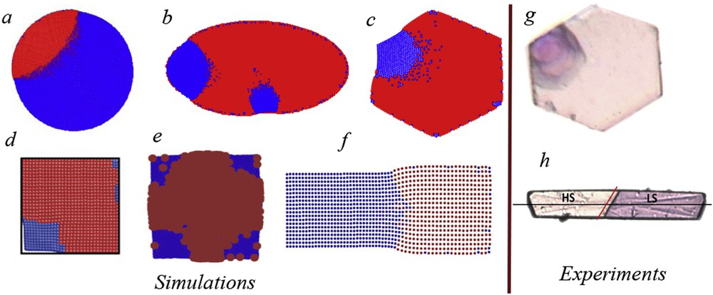
Clusters of LS molecules in an HS background spread from edges in circular and elliptic samples and from corners in hexagonal- and rectangular-shaped systems. Simulations have been made using molecular dynamics modelling (a, adapted from Ref. [38]), mechanoelastic model with Arrhenius and Metropolis probabilities, (b and c, adapted from Refs. [45] and [44], respectively), two-variable elastic Ising-like model (d, adapted from Ref. [47]), electroelastic model (e and f, adapted from Refs. [39] and [40], respectively). Comparison with experimental data, obtained by optical microscopy (g and h, adapted from Refs. [18] and [23], respectively).

Fig. 4
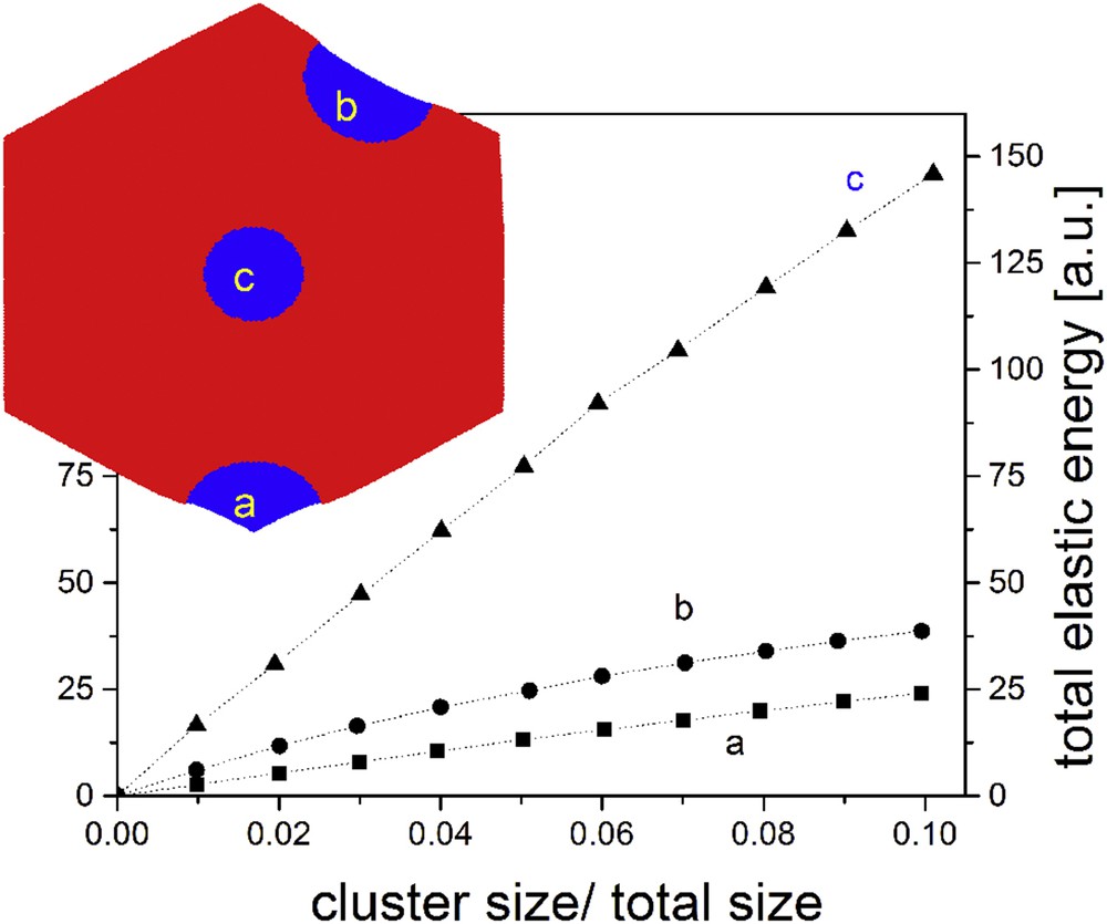
Example of the increase in the elastic energy of the system for clusters starting from a corner (a), the hexagon edge (b) or the hexagon centre (c), characterized by a π/2 contact angle.

The cluster spreading in such elastic systems has been discussed in the framework of the “macroscopic nucleation” [38] concept, which can be extended for other systems exhibiting long-range interaction and which implies that the size of the critical nucleus is proportional to the system size. During the propagation process, the existence of three regimes has been identified: the incubation, corresponding to the initial formation of a cluster; the flow, corresponding to a linear velocity of the cluster; and the acceleration, corresponding to the last stages of relaxation when the opposite surface is close. The study of the speed dependence on the elastic constant has shown that the speed is lower for more rigid lattices [40]. This can be correlated to the larger velocity experimentally observed in many cases for the heating process, with respect to the cooling process [23]. In addition, it was stated [23] that the interface velocity is a monotonous function of temperature, passing through zero at the equilibrium temperature and if the temperature is constant its evolution cannot be reversed. One should distinguish between the interface propagation and the propagation of elastic interactions, as it was experimentally shown that the domain propagation is much slower than the propagation of sound waves [23]. This feature is particularly important for ultrafast phenomena, where the volume variation does not exactly follow the variation in the $n_{HS}$ fraction, due to different times needed for cluster spreading and for the propagation of elastic distortions towards the edges of the system [26,52].

Excepting a small part distributed at the surface of the lattice, the elastic energy at equilibrium, as well as the higher local pressures, is located at the interface between the two phases [24,40,47]. However, the value of this elastic energy almost vanishes for specific orientations of the border lines, as it was demonstrated by an anisotropic extension of the electroelastic model, which took into account the atomic structure of the crystal via a simple one-site model [24]. Comparable evidence results from the analysis of the maps of the local pressures, which correspond to local deformation fields in a continuous medium. Similar to higher local pressures, higher strain can be detected at the interface between the two phases (see Fig. 5). Therefore, for a fixed size of a cluster, the most stable interface shape is that with the shortest length, and both electroelastic and mechanoelastic models confirmed that the contact (wetting) angle between the interface and the lattice border must be around $π / 2$ . For example, in the case of a circular lattice, the nucleation starts at the edge of the lattice with a circular shape, which gradually changes through the propagation, becoming a straight line at the middle of the region, whereas the interface length is maximal and returning to a circular shape towards the end of the process with a decrease in the interface length.

Fig. 5
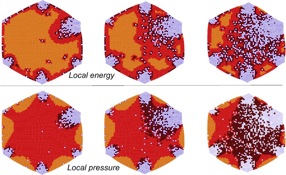
Instabilities at the interface border in terms of local energies (up) and local pressures (down). LS molecules: blue open circles. HS molecules: dark red circles in the case of high energy (pressure), red circles in the case of average energy (pressure), light red circles in the case of low energy (pressure). The instability is larger for darker circles.

3.2 Finite size effects

3.2.1 Introduction

In the last decade, an intense research activity has focused on the investigation of the size reduction effect on the physicochemical properties of all classes of switchable molecular materials or coordination networks, with a special attention to SCO systems [69] and Prussian blue analogue (PBA) coordination polymers [70]. In particular, the understanding of the phase transition mechanism at the nanometric scale and the control of the phase stability is of paramount importance for their future potential applications in memory and display devices as molecular switches or in SCO strain-based systems [71].

It is important to note that strictly speaking, a phase transition only exists in the thermodynamic limit, that is, when the number of degrees of freedom and the volume are infinite, their ratio remaining constant. Phase transitions are because of the existence of latent heat or singularities in the Gibbs energy, which produce divergences or discontinuities of their derivatives (order parameters, susceptibilities, etc.). Finite size effects remove such singularities, and thermodynamic or statistical physics approaches introduced for large systems may not be suitable for smaller systems any more. However, for clarity reasons, we abusively call “phase transition” any phase transformation or spin state changes observed at finite sizes.

Common features exist in the size dependence of physical, chemical and thermodynamic properties in different materials in condensed and soft matter ([72] and references therein). In general, size reduction effects are characterized by the occurrence of two phenomena. First, finite size effects lead to confinement effects, which can affect transport phenomena (electrical, mechanical, optical, etc.) and more generally any collective behaviours. It leads to various quantum physical phenomena and cavity effects. On the other hand, the increase in the surface-to-volume ratio, resulting in the predominance of surface/interface properties, modifies mostly the phase stability and phase transformation kinetics. The typical size below which sizeable modifications appear in transport processes, physical and chemical properties and thermodynamic quantities are largely dependent on the structural characteristics of the material, the observed physical phenomenon, the measured observables (magnetization, thermal or/and electrical conductivity, electric polarization, etc.) and the transport mechanism (delocalized electron, acoustic phonons, dislocations, etc.) related to this phenomenon. Moreover, the different phenomena we usually consider as size effects do not take place at the same size range: although modifications of nucleation and domain growth processes may occur at the micrometre scale, quantum confinement effects are expected to be noticeable in very small systems (few nanometres). In the following, the different theoretical approaches and the fundamental concepts introduced to reproduce the experimental observations in SCO nanomaterials are overviewed.

3.2.2 Surface effects: description with local physical property modifications

In a pioneering work, Kawamoto and Abe [73] have pointed out the importance of the surface in the spin transition properties of small systems. The well-known Ising-like model has been treated by Monte Carlo simulations on cubic and spherical systems with open boundary conditions (OBCs). In comparison with periodic boundary conditions (PBC), they showed that the hysteresis width decreases with size reduction in a different manner according to the nanoparticle shape, whereas the phase stability (in particular the equilibrium temperature) remains size independent (Fig. 6). The different observations were attributed to different nucleation processes existing in cubic and spherical systems and to the decrease in the number of interacting molecules when approaching very small systems.

Fig. 6
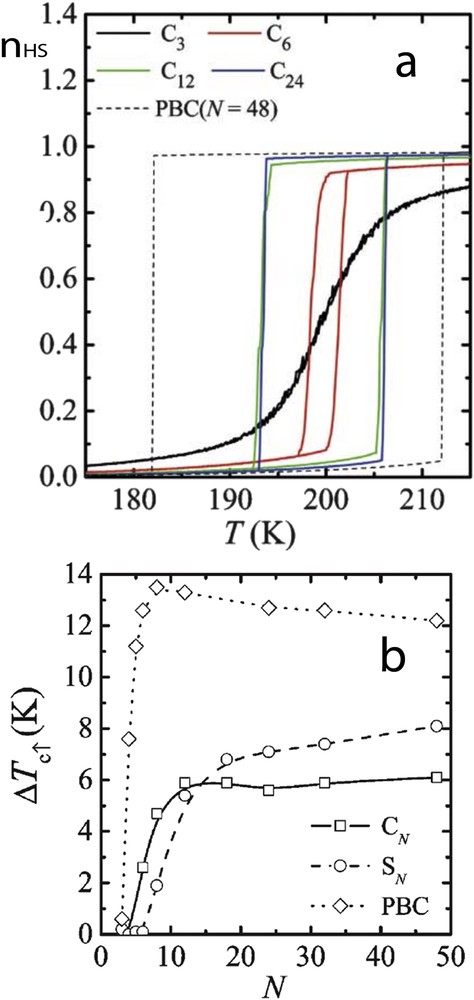
(a) The fraction of the unit in the HS state in an equilibrium state, n_H, for various sizes of cubic particles. For comparison, the result at N = 48 with the PBC is also shown. (b) Size dependence of the width of the thermal hysteresis ΔT_c for cubic particles (C_N), spherical ones (S_N) and the PBC case.

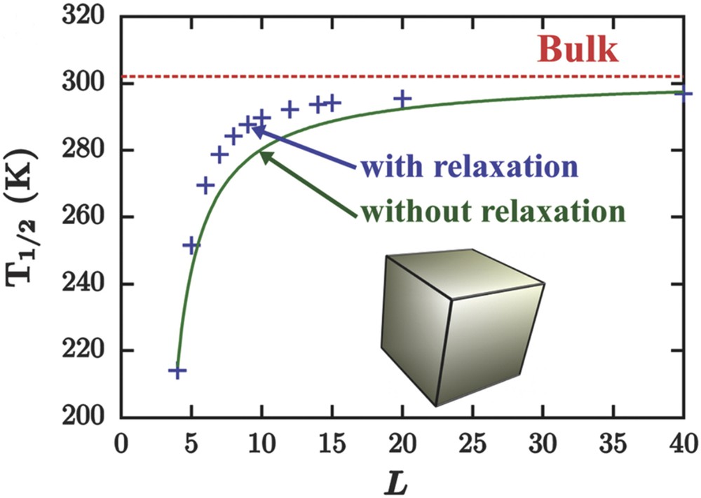
However, experimental observations in some coordination nanoparticles have brought out a strong size dependence of the phase stability, which results in a downshift of the equilibrium temperature and the presence of incomplete transitions [74,75]. Indeed a number of residual HS molecules in the nanoparticles remain at low temperature and the associated HS fraction increases with the rise in the surface-to-volume ratio suggesting the presence of inactive molecules at the surface. The origin of inactive molecules at the surface with different physical and chemical properties may be attributed to surface chemical reactions, structural disorder and/or the alteration of the ligand by the external environment. This finding has been taken into account by adding specific boundary conditions (surface molecules fixed in the HS state [76] or a weakening of the ligand field at the surface [77,78]). The investigation of local surface effects in squared nanoparticles using the Ising-like model with such specific boundary conditions (surface molecules fixed in the HS state) has demonstrated that the HS surface sheet acts as a “negative pressure” [76] (nb: lattice deformations are not explicitly taken into account in the Ising-like model), but pressure effects can be grasped through an effective modification of the ligand field [76]. This leads to a downshift in the equilibrium temperature, which follows an algebraic law with the size (Fig. 7):

T_{eq} = T_{eq} (\infty) - \frac{8 J}{k_{B} \ln (g)} \times \frac{1}{L - 2}

(27)

where L is the side length of the square nanoparticle and T_eq(

\infty

) is the equilibrium temperature of the bulk material. This algebraic decay seems to be a universal feature of the size evolution of the phase stability and has been already observed in other first-order transitions such as melting process in bimetallic nanoparticles [79].

Fig. 7
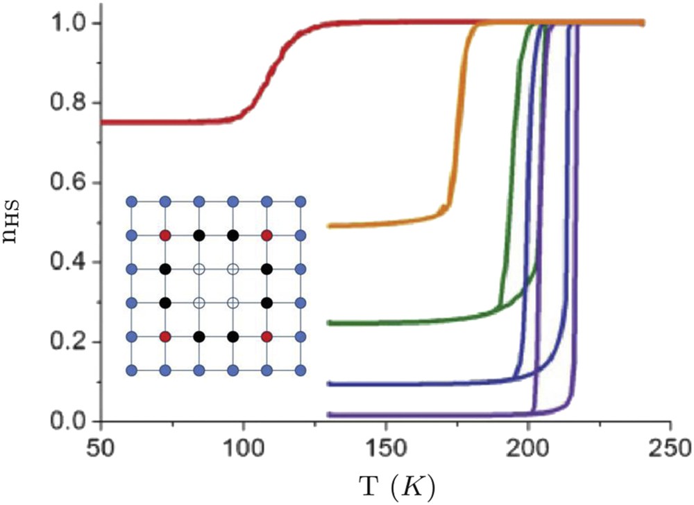
Calculated temperature dependence of the HS fraction for square-shaped nanoparticles of different sizes in the framework of the Ising-like model with fixed boundary conditions (HS state fixed at the surface). From left to right, L = 4, 7, 10, 40, 200 (quasi-infinity). Insert: Lattice configuration in the case L = 6. Blue filled circles are HS-fixed (edge) atoms. All inside atoms are active: filled red (black) circles stand for atoms having two (one) inactive HS as nearest neighbours, and open circles stand for atoms surrounded by only active sites.

The presence of surface physical properties different from those of the nanoparticle core has been formulated in terms of surface energies in a simple nanothermodynamic model [80]. Surface energy is a physical ingredient experimentally accessible and despite the fact that different physical and chemical contributions are involved behind this concept, the thermodynamic approach remains a powerful tool to make direct comparisons with experimental observations [81]. Let us consider a spherical SCO nanoparticle with a radius R constituted of a bulk-like core, which is connected to a surface A, the so-called core–shell approach. This core–shell nanoparticle is in contact with a thermostat and a barostat and the Gibbs free energy G can then be written as an extension of the Slichter and Drickamer model:

G = n_{HS} G_{HS} + (1 - n_{HS}) G_{LS} - T (S_{mix}^{b} + S_{mix}^{s}) + A (σ_{HS} n_{HS}^{s} + σ_{LS} (1 - n_{HS}^{s})) + Γ (1 - n_{HS})

(28)

where

G_{HS}

and

G_{LS}

stand for the Gibbs free energy of the HS and LS phases, respectively.

S_{mix}^{b}

and

S_{mix}^{s}

are, respectively, the mixing entropies of the core and the shell assuming there is no diffusion of molecules from the bulk to the surface of the nanoparticles. Γ is a phenomenological parameter, taking into account interactions between molecules. σ_HS and σ_LS correspond to the surface energy density costs for the creation of an HS and an LS surface, respectively. This approach is less restrictive than fixed boundary conditions according to the difference between σ_HS and σ_LS, the size reduction leads either to a downshift (σ_HS < σ_LS) or an upshift (σ_HS > σ_HS) of the transition temperature (Fig. 8b). The latter follows the same algebraic decay as presented in Ref. [76] (Fig. 8a), when the nanoparticle radius is reduced. When the difference

Δ σ

becomes important, incomplete transitions occur at low or at high temperatures. In this latter situation, molecules at the surface become inactive and the fixed boundary conditions proposed in Ref. [77] are retrieved; however, the possibility to fix the surface in the LS state is not excluded.

Fig. 8
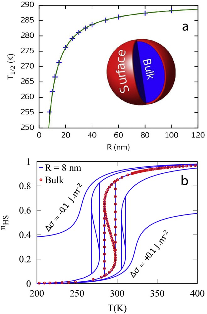
(a) Evolution of the equilibrium temperature with the size reduction. Insert: schematic representations of a spherical core–shell nanoparticle; (b) simulation of spin transition curves with the nanothermodynamic model. The symbols display the spin transition for the bulk material. The lines show the transition for an 8 nm nanoparticle with different surface energy density differences between the HS and LS phases Δσ = σ_HS − σ_LS.

Two main conclusions emerge from this nanothermodynamic model. First, the surface energy can be seen as the driving force of the spin transition at the nanoscale. Then, the downshift of the transition temperature with the occurrence of a residual HS fraction at low temperature in small nanoparticles seems to be the most common observation in SCO coordination nanoparticles, even if an upshift of the transition temperature and residual LS fraction have also been reported [81]. From a microscopic point of view, less constrained boundary conditions have been applied in the framework of Ising-like [82], anharmonic [72] and electromechanical [83] models, considering that chemical and physical (ligand field, vibronic degeneracies, elastic constant and lattice parameters) properties of the surface are different from those of the nanoparticle core.

Beyond the different theoretical descriptions used with the aim to model surface effects, a more fundamental question to ask is “what can be the mechanisms and the associated relevant chemical and physical ingredients at the origin of the different experimental observations?” In surface physics, it is well known that the first trivial consequence of the surface creation is the emergence of coordination defects: the local environment at the surface is different from the core due to broken bonds. Broken LS bonds cost more energy than HS bonds, which results in a stiffer lattice in the LS phase than in the HS phase at a macroscopic level. In Ref. [74], the surface energy density related to the coordination defect of a squared lattice has been expressed as a function of the bond energy of nearest- and next nearest-neighbour molecules:

σ = \frac{- v_{1} - 2 v_{2}}{2 r} - \frac{v_{1}}{\sqrt{V}}

(29)

where v₁ and v₂ are the cohesion energies of nearest- and next nearest-neighbour molecules, respectively, r is the side of the squared lattice and V its “volume”. Because the cohesion energy of the LS lattice is stiffer (v_HS < v_LS), from Eq. (29) we can deduce that the coordination defect tends to favour the HS state at the surface (σ_HS < σ_LS). Interestingly, this is not enough to explain the drastic change in the phase stability of coordination nanoparticles.

The simulation of hollow SCO nanoparticles with the anharmonic spin–phonon model has highlighted the importance of the surfaces on the spin transition properties: rather than the quantity of matter, it is the surface-to-volume ratio that counts [77]. Indeed, a filled nanoparticle and a hollow nanoparticle having largely different volumes (i.e., different number of molecules) but the same surface-to-volume ratio exhibit similar spin transition curves.

3.2.3 Surface effects: surface and order parameter relaxations

Surface relaxations or/and surface structural reconstructions, which accompany most of the time coordination defects, cannot be neglected in the modelling of the spin transition at the nanoscale. Therefore, the theoretical investigation of size reduction in SCO materials with models taking explicitly into account lattice degrees of freedom and elastic deformations becomes indispensable. Monte Carlo simulations in the (N,P,T) ensemble using a spring–ball Hamiltonian on a cubic lattice have shown that surface physical properties are delocalized in the core due to the surface–bulk mechanical coupling [84]. In other words, the approximation of a surface without depth may not be correct. Indeed, profiles of the mean squared displacement for different nanoparticle sizes show that below a critical size L_c (ca. L_c ∼ 7–8 nm in this case) the vibrational and elastic properties of the nanoparticle become completely different in comparison with the corresponding bulk materials.

The calculated Debye temperature and the melting temperature drastically decrease below L_c in the case of free surfaces, which can be understood by the fact that molecules at the surface can move more easily than those in the bulk and have the higher mean squared displacement and also a lower Debye temperature. On the contrary, when specific boundary conditions are imposed by ad hoc increasing the elastic constants of surface bonds, the Debye temperature increases with the size reduction.

Free surfaces seem to have only a relatively weak effect on the phase stability: the transition temperature remains nearly size invariant and no residual HS fraction occurs by approaching the nanometre size. The modelling and the prediction of the surface structural relaxation is rather complicated because different contributions, such as the coordination number, the crystallographic properties of the materials and so forth are involved in this phenomenon. However, two kinds of surface relaxations can be distinguished: surface structural relaxations and order parameter relaxations. In this present case, the order parameter of the spin transition is the HS fraction, $n_{HS}$ . The electron–lattice coupling in SCO materials does not allow one to independently study these two contributions. Therefore, surface relaxations have been investigated within the framework of the Ising-like model. The decomposition of the free energy of an SCO chain has been proposed in the framework of a 1D Ising-like model, solved by transfer matrix techniques [85], comparing open and periodic boundary conditions. In this work, a detailed analysis of the bulk, the surface and the finite size effects on the thermodynamic properties has highlighted that the contribution of the finite size effects in free energy is always smaller than that of the surface free energy.

A similar 3D Ising-like model has been solved in the inhomogeneous mean-field approximation in which only spin-state surface relaxations are present [86]. The different surface thermodynamic quantities have been extracted as follows:

\begin{array}{l} F_{Σ} = F - F_{B} = F_{Σ}^{MB} + F_{Σ}^{relax} + F_{Σ}^{size} \\ E_{Σ} = E - E_{B} = E_{Σ}^{MB} + E_{Σ}^{relax} + E_{Σ}^{size} \\ S_{Σ} = S - S_{B} = S_{Σ}^{MB} + S_{Σ}^{relax} + S_{Σ}^{size} \end{array}

(30)

where the surface free energy

F_{Σ}

, the surface internal energy

E_{Σ}

and the surface entropy

S_{Σ}

are defined as excess quantities in comparison with the corresponding thermodynamic variables of the infinite system. The main advantage of the inhomogeneous mean-field Ising-like model resides in the possibility to separate the contribution of the coordination defect, the so-called missing bond (

X_{Σ}^{MB}

), from the spin-state surface relaxations (

X_{Σ}^{relax}

), because finite size effects

X_{Σ}^{size} = 0

do not exist in the framework of mean-field approaches. Overall the surface relaxations partially attenuate the effect of the coordination defects, in particular, the expensive energy cost for the breaking of bonds (Fig. 9).

Fig. 9
Size evolution of the equilibrium temperature of an Ising-like model treated in the framework of homogeneous (missing bonds, full green line) and inhomogeneous (missing bonds, surface relaxations, blue crosses) mean-field approximation. The transition temperature in the thermodynamic limit (bulk red dashed line) is represented as a reference.

Interestingly, when the evolution of the surface thermodynamic quantities is inspected, two findings can be established. Far from the transition temperature(s), the main contribution to the surface thermodynamic quantities comes from the coordination defect. However, around the transition temperatures, spin-state surface relaxations become non-negligible and compete with the coordination defects. However, in system exhibiting first-order transition (and also second-order transition), the surface relaxation effects become predominant mainly because bulk–surface correlation length massively increases (diverges) approaching the HS–LS coexistence region (the critical point).

Surface relaxations have also been investigated by considering a hexagonal lattice in which the unit cell contains two different sites: an active SCO and an inactive site. The aim was to mimic a simplified structure of the coordination network [Fe(pyrazine)(Ni(CN)₄)] with an elastic anharmonic model [87]. The inactive site tends to favour the LS state by exerting a compressive local stress on the active site in the nanoparticle. This stress is relaxed at the surface where a tensile stress exists, favouring the HS state. The nanoparticle exhibits a two-step spin transition where the active molecules at the surface switch at a lower temperature than those located in the core and can be seen as an incomplete transition if the temperature is not sufficiently decreased (Fig. 10). Remarkably, in this study, no specific boundary conditions are imposed. The particular structure combined with OBCs leads to the emergence of this two-step transition. Interestingly, in the frame of this “elastic” model, contributions from structured and spin-state relaxations to the total surface relaxation could be separated.

Fig. 10
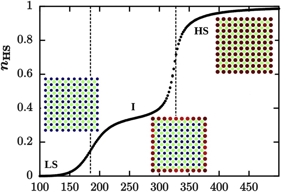
(a) Spin transition curve of a nanoparticle containing both active and inactive sites in a squared lattice simulated with the anharmonic model investigated by Monte Carlo methods. The presence of an inactive site in the structure generates internal stresses, which relax at the surface, leading to a two-step transition with the occurrence of an intermediate state I, constituted of HS molecules close to the surface and LS molecules in nanoparticle core. The surface tensile stress favours the HS state at the surface and therefore sites at the surface switch at a lower temperature than sites localized in the nanoparticle core.

3.2.4 Impact of size reduction on cooperativity and collective elastic behaviour

An important question concerns the bistability property at the nanoscale. Can the hysteretic behaviour be observed in ultrasmall nanoparticles? This point is very important for the integration of SCO materials in information storage devices and other applications involving a memory effect. In a first approach, the disappearance of the hysteresis was predicted because of the decrease in the number of interacting molecules and the large fluctuations existing in a system containing a limited number of degrees of freedom. By analogy with magnetic nanoparticles, a phenomenon similar to superparamagnetism was expected in SCO nanoparticles. The first theoretical investigations of size effects using the Ising-like model support this assumption [73]. Whatever the numerical (Monte Carlo) or analytical (mean-field approximation) treatment of the Ising-like model and despite some differences because of the presence of short- or long-range interactions in the nanoparticle, a shrink of the hysteresis loop is generally observed with the size reduction [76,78]. However, experimental observations have shown the presence of hysteretic behaviour in the spin transition curves of some rather small SCO nanoparticles. Among different possible explanations, the size-dependence of the lattice stiffness has been evoked. Indeed, the size dependence of the Debye temperature $θ_{D}$ extracted from Mössbauer data in PBA and SCO coordination networks have revealed a stiffening of particles below ca. 5 nm (Fig. 11a). Inserting these experimental findings in the phenomenological interaction parameter $Γ$ of the nanothermodynamic model ( $Γ \sim θ_{D}^{2}$ ), a nonmonotone size evolution of the hysteresis width is observed: for intermediate nanoparticle sizes the hysteresis loop shrinks and disappears before reappearing in very small nanoparticles (Fig. 11b) [80].

Fig. 11
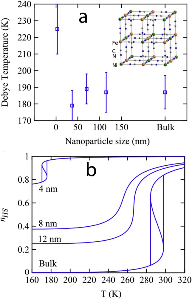
(a) Size evolution of the Debye temperature for Ni₃[Fe(CN)₆] PBA nanoparticles extracted for ⁵⁷Fe Mössbauer spectroscopy measurements. (b) Spin transition curves for different nanoparticle sizes calculated with the thermodynamic model (Eq. (28)), taking into account the experimental observation of nanoparticle stiffening with the size reduction.

This result is in good agreement with experimental observations. The concept of cooperativity is upset by approaching the nanometer scale. There are less interacting entities in SCO nanoparticles, but it may be compensated by stronger bonds. A word of caution is needed here. Indeed, it is not obvious that the elastic theory remains valid in such small nano-objects and quantities such the Debye temperature and the bulk elastic modulus become meaningless. Another important point is the intrinsic character of the elastic/vibrational properties of a solid. Such quantities are not expected to be size dependent and the apparent or effective stiffening arises likely due to a compressive stress exerted by the external environment. The different effects of the environment are discussed in section 3.2.5. Another assumption to explain the observation of the bistability in nanoparticles is the presence of kinetic effects. Indeed, nanoparticles cannot reach the thermodynamic equilibrium because they are constantly crossed by heat and mechanical flows. Any small perturbations can destabilize the nanoparticle stationary state. The nanoparticle may switch permanently and very quickly from one state to another like in superparamagnetism. In this case, the existence of hysteresis has a kinetic origin and only the average time spent by the nanoparticle may be observed.

3.2.5 Matrix effects (external environment)

Analogue to the Ising-like models mentioned above, the classical elastic models applied for open boundary SCO systems led to same unsatisfactory results: only the less steep transition and the smaller hysteresis, which vanishes for a critical size, could be reproduced. A different approach to account for all experimental features consisted in considering samples embedded in a polymer surrounding environment [88]. The motivation for this approach resides in the fact that some methods of preparation of nanoparticles imply the use of either the inverse micelle method or the polymer protected synthesis to obtain different particle sizes. The polymer itself forms a more or less flexible matrix around the nanoparticles, preventing the agglomeration of nanoparticles to form larger ensembles. The SCO molecules at the surface will therefore interact with the polymer matrix via either van der Waals interactions or hydrogen bonding. In a first approach, the systems used in the Ising-like model have been modified by considering an embedding matrix of nonswitching molecules, interacting with edge SCO molecules [78]. The results have satisfactory reproduced experimental data, but for a more realistic approach, the use of elastic models has been necessary. The polymer is represented in this approach as a rigid or flexible shell of nonswitching molecules, which interact with the molecules situated at the edge of the lattice by way of springs, with a given elastic constant denoted as k_pol. When the HS to LS transition occurs, the SCO nanoparticle shrinks, and if the polymer is not flexible enough, an increasing negative pressure appears at the edge of the system, originating in pulling forces from the polymer network. With this premise, the hysteresis not only shifts to lower temperatures, but also for high enough interactions between edge molecules and polymer, a residual HS fraction is produced (Fig. 12).

Fig. 12
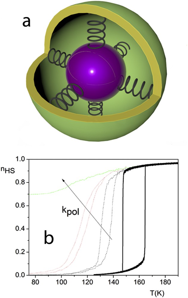
Elastic particles linked by springs to a matrix (a) and the effect on the thermal transition for different values of k_pol (b).

Similar results have been obtained with an Ising-like model containing a long-range interaction terms. The interaction with the external environment has been taken into account through a short-range coupling term between surface SCO molecules and the matrix containing inactive HS molecules. If the Ising coupling is strong enough, the molecules at nanoparticle surfaces are fixed in the HS state. Very recently, the experimental and theoretical investigations of physical properties of hybrid nano-objects and hollow nanoparticles have known a growing interest for practical and fundamental reasons. Indeed, SCO hybrid nano-objects, especially core–shell nanoparticles, allow a control of the spin transition properties and permit to generate synergies between the physical properties of the core and the shell (optical, magnetic, electric, elastic, etc.), which makes them particularly interesting for technological applications. On the other hand, these objects are very suitable for the fundamental investigations of the role of the external environment and interfacial interactions on the phase stability at the nanoscale. Monte Carlo simulations using the electrovibrational model have been performed by Oubouchou et al. [83] considering a nanoparticle embedded in an external environment whose elastic properties and structure were chosen to be similar to the HS phase (“soft” matrix). The analysis of the strain and local pressure mappings show that increasing the thickness of the surrounding medium leads to a release of the elastic strain at the interface nanoparticle/matrix and a decrease in the transition temperature (Fig. 13).

Fig. 13
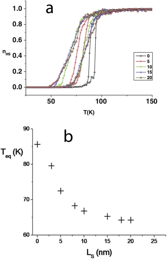
(a) Thermal dependence of the HS fraction for square-shaped nanoparticles at constant core size surrounded by a various number of HS shell layers (0–20). The hysteresis shifts downwards as a result of the negative elastic pressure induced by the shell. (b) Evolution of the equilibrium temperature for different shell thickness (L_s).

On the basis of a similar approach, Slimani et al. have demonstrated that the external matrix permits to maintain the bistability property in the SCO nanoparticle if the matrix/nanoparticle couplings are strong enough [41]. A further extension of the electroelastic model has been used to simulate SCO heterostructures [89]. In particular, the thickness and the rigidity influence of the surrounding shell on the spin transition properties of the core have been investigated by Monte Carlo simulation. The shell rigidity strongly affects the thermal hysteresis of the SCO core. In addition, resonance behaviour is observed when the shell rigidity is close to that of the core (Fig. 14).

Fig. 14
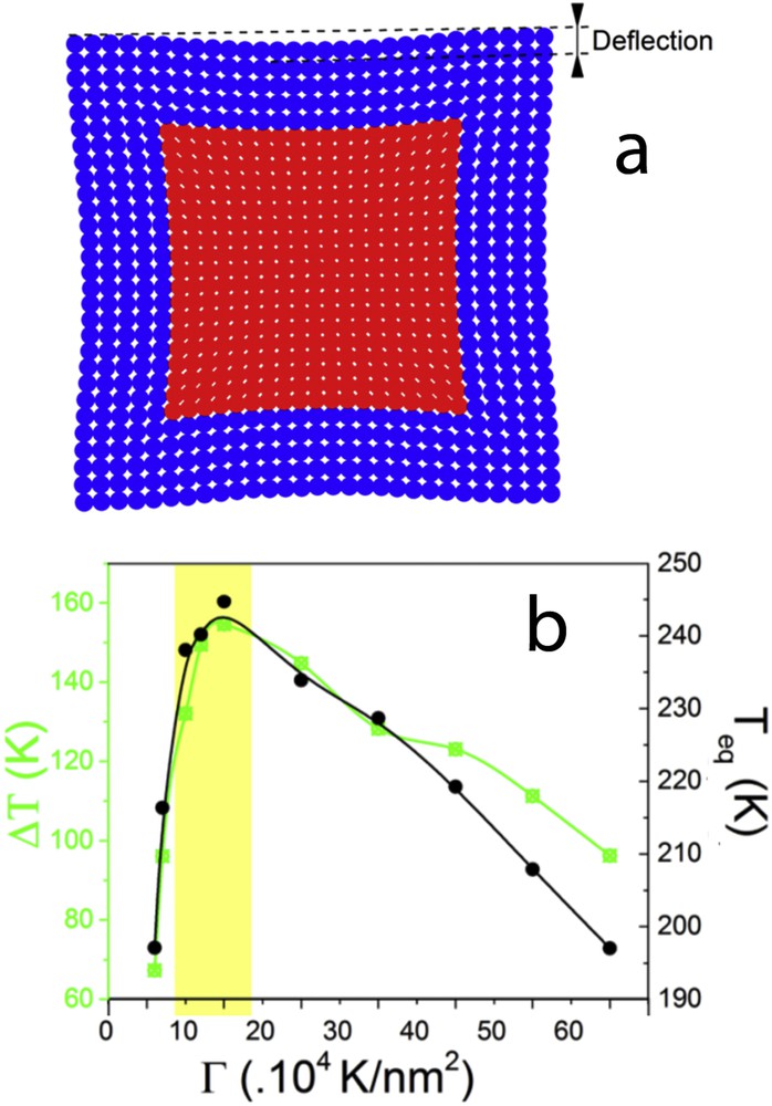
(a) Example of a simulated squared core–shell nanoparticle using the electroelastic model. The elastic misfit between the core and the shell induces a strain in the heterostructure, which can be quantified by the calculation of the deflection. (b) Effect of the shell stiffness on the thermoinduced spin transition of the core–shell nanoparticle: hysteresis width (green line) and equilibrium temperature (black line).

Félix et al. have simulated core–shell nanoparticles using the spin–phonon model solved by the Monte Carlo simulations [77]. The control of the transition temperature of the hybrid nanoparticles can be achieved by tuning the elastic misfit (lattice parameters) between the core and the shell. When the core and the shell have similar elastic properties, the interfacial energy is zero and no phase stability change is observed in comparison with the corresponding nanoparticle or hollow nanoparticle. When the elastic misfit generates a compressive (respectively tensile) stress on the SCO core, an upshift (respectively downshift) of the transition temperature is observed. Interfacial energy is minimized when the core is in the LS state (respectively HS state). Interestingly, when an active core (e.g., SCO materials) is coupled with a shell sensitive to mechanical stress (e.g., martensitic materials) through a sufficiently coherent interface, a novel kind of hysteresis effect can be generated; the transition temperature is upshifted (respectively downshifted) during the warming (respectively cooling) process.

Despite elastic models give an origin of the core–shell coupling mechanism, it remains difficult to establish a link between the Hamiltonian parameters and experimentally accessible quantities. Therefore, an analytical approach modelling a core–shell nanoparticle with a coherent interface using continuum medium mechanism has been developed [90]. Analytical expressions of the interfacial stress $(P_{in})$ and the interfacial elastic energy density have been derived as a function of the Young's moduli (Y), the Poisson ratio ( $ν$ ) as well as the size (a, b) of the core (subscript 1) and the shell (subscript 2):

P_{in} = \frac{2 b^{2} a_{2} \frac{1 - υ_{2}^{2}}{Y_{2} (b^{2} - a_{2}^{2})} + a_{1} - a_{2}}{\frac{a_{1}}{Y_{1}} + (1 + υ_{1}) (1 - 2 υ_{1}) + \frac{a_{2}}{Y_{2}} \frac{1 + υ_{2}}{(b^{2} - a_{2}^{2})} [(1 - 2 υ_{2}) a_{2}^{2} + b^{2}]}

(31)

See Fig. 15 for the definition of a₁, a₂ and b.

Fig. 15
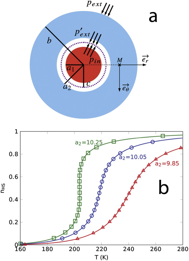
(a) Scheme of an elastic circular core–shell particle. Lengths a₁ and a₂ represent the radius of the core and that of the shell hole, respectively. Length c represents the radius when the core and hole surfaces are in contact ( $a_{1} = a_{2}$ ). The pressure exerted by the core on the shell is the same as the pressure exerted by the shell on the core, $P_{in} = P_{ext}^{'}$ ; (b) Spin transition curves of SCO nanoparticles with an inactive shell simulated by a thermodynamic model taking into account the core–shell interfacial elastic energy model. When an elastic misfit exists between the core and the shell, the elastic interfacial energy favours either the HS state (green squares) or the LS state (red triangles) depending on the sign of the misfit, whereas the spin transition curve remains unchanged in comparison with an isolated nanoparticle in the absence of misfit (blue circles).

A quantitative investigation of the impact of the interfacial elastic energy on the phase stability can also be performed to optimize the elastic coupling between the core and the shell. The spin transition of the core–shell nanoparticle can be simulated by injecting the interfacial energy density into the nanothermodynamic model. It is important to note that the role of the elastic misfit on the collective behaviour and the bistability cannot be grasped with this model, because the elastic interaction between molecules is not explicitly taken into account in the Slichter and Drickamer [4] model and also the elastic interfacial stress cannot be coupled with the distortions occurring during the spin state change. This constitutes the main drawback of this approach.

3.2.6 Consequences on thermodynamic quantities and vibrational properties

Size reductions have usually a strong impact on the thermodynamic properties of materials. The increasing role of surface (interface) thermodynamic properties destroys the postulates from which classical thermodynamics are built. For instance, thermodynamic quantities or functions are no more proportional to the quantity of matter and become nonextensive. This has been highlighted through the investigation of size dependence of internal energy and entropy of a spring–ball system calculated with histogram Monte Carlo methods (Fig. 16) [77].

Fig. 16
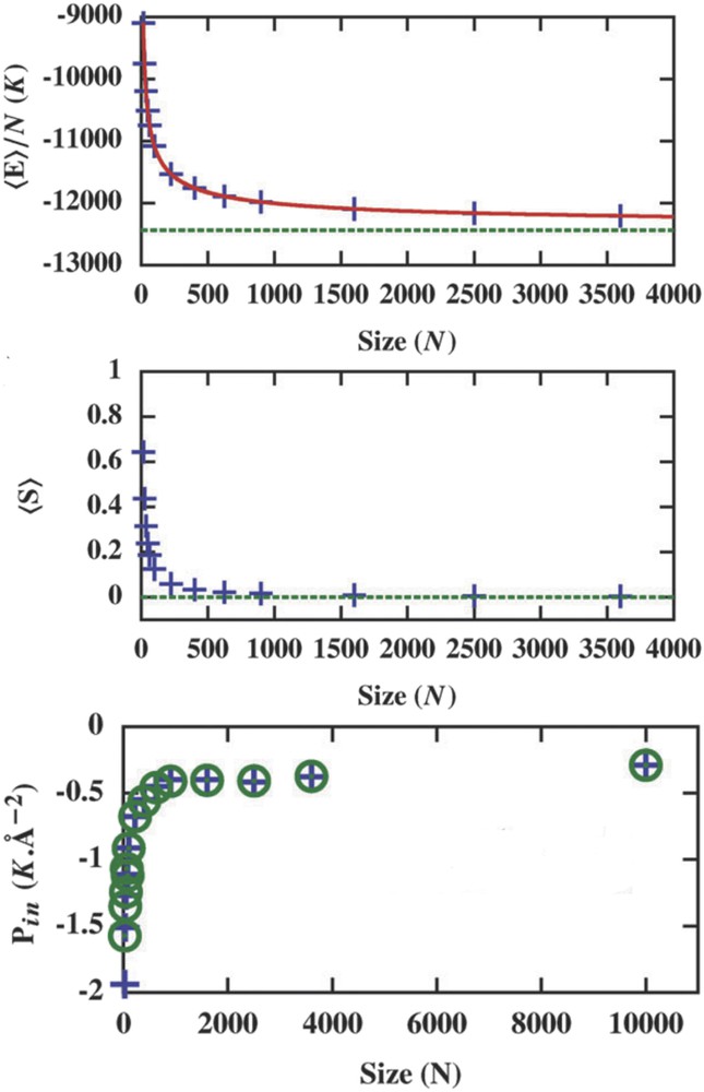
Energy per site (a) and entropy per site (b) as a function of the total number of sites (crosses) with the infinite value (horizontal dotted line) calculated by the Monte Carlo simulation. (c) Size dependence of the internal pressure P_int of the particle at the external pressure P_ext = 0 K Å⁻².

As mentioned above, the thermodynamic equilibrium cannot be reached and even a perfect thermostat and a perfect barostat can no more impose its temperature and pressure, which are no longer intensive quantities. As a consequence, the external and internal pressures are related by a Young-Laplace–like relation, which can explain the apparent change in the nanoparticle stiffness:

P_{in} = P_{ext} - \frac{2}{\sqrt{V}} - 4 \sqrt{V} \frac{\partial σ}{\partial V}

(32)

where V is the volume and σ is the surface energy density. The nonextensive character of thermodynamic quantities (internal vibrational energy and vibrational entropy) at the nanoscale has been very recently highlighted through nuclear inelastic scattering experiments in SCO coordination nanoparticles [91]. Molecular dynamic simulations of the size dependence of vibrational properties of nanostructures taking into account the octahedral symmetry of the SCO complex have shown that the change in the density of vibrational states cannot be attributed to confinement effects but rather to surface/matrix effects [92]. Nevertheless, some aspects concerning the behaviour of the thermodynamic functions approaching the nanometre scale remain unclear, in particular the increase in the vibrational entropy and vibrational internal energy, which is not expected in unstressed nano-objects constituted with less chemical bonds than the massive material (free boundary conditions). The discrepancy between experiments and simulations can be due to the size and/or shape distribution of nano-objects, which tends to mask quantification effects. Deeper investigations of the lattice dynamics of SCO nanoparticles have to be performed considering the morphology and the polydispersity of the samples. Matrix effects have to be included in molecular dynamics through the application of additional constraints (force fields) on the surface of the modelled nanostructures. However, this requires a more precise knowledge of the chemical nature of the coupling between the external environment and the nanoparticles.

4 Conclusions

Elastic models constitute a step forward for the understanding of the behaviour of cooperative SCO materials. Largely improving previous models, they are, in all their different but convergent forms, both more precise and realistic than mean-field or Ising-like models used for simulating phenomenological behaviours of bulk SCO compounds and faster than ab initio approaches used for finding the electronic and bonding states on single molecules. They are able to reproduce both macroscopic curves and microscopic evolutions in bulk materials and also to simulate finite size effects for nano- and microparticles, with OBCs or embedded in surfactants. Future challenges for these models should include the simulations on structure compatible to real samples, either 2D or 3D, with the final aim to integrate real parameters found in ab initio models.

Acknowledgements

We thank Dr. Gabor Molnàr for carefully proofreading the manuscript and for his useful comments. W.N. and C.E. thank, respectively, to CNRS France and UEFISCDI Romania for research grants.

Bibliographie

[1] A. Bousseksou; J. Nasser; J. Linares; K. Boukheddaden; F. Varret J. Phys. I France, 2 (1992), pp. 1381-1403

[2] K. Boukheddaden; J. Linares; H. Spiering; F. Varret Eur. Phys. J. B, 15 (2000), p. 317

[3] T. Kambara J. Chem. Phys., 70 (1979), p. 4199

[4] C.P. Slichter; H.G. Drickamer J. Chem. Phys., 56 (1972), pp. 2142-2160

[5] J.D. Eshelby Solid State Phys., 3 (1956), pp. 79-144

[6] H. Spiering; E. Meissner; H. Koppen; E.W. Muller; P. Gütlich Chem. Phys., 68 (1982), pp. 65-71

[7] T. Kambara J. Chem. Phys., 74 (1981), pp. 4557-4565

[8] R. Zimmermann; E. Konig J. Phys. Chem. Solids, 38 (1977), p. 779

[9] J. Jung; G. Schmitt; L. Wiehl; A. Hauser; K. Knorr; H. Spiering; P. Gutlich Z. Phys. B, 100 (1996), pp. 523-534

[10] J. Nasser Eur. Phys. J. B, 48 (2005), p. 19

[11] J. Nasser; S. Topcu; L. Chassagne; M. Wakim; B. Bennali; J. Linares; Y. Alayli Eur. Phys. J. B, 83 (2011), pp. 115-132

[12] M. Sorai; Y. Maeda; H. Oshio J. Phys. Chem. Solids, 51 (1990), p. 941

[13] E. Konig; B. Kanellakopulos; B. Powietzka; J. Nelson J. Chem. Phys., 99 (1993), p. 9195

[14] C. Enachescu; H.C. Machado; N. Menendez; E. Codjovi; J. Linares; F. Varret; A. Stancu Physica B, 306 (2001), p. 155

[15] G. Molnár; A. Bousseksou; A. Zwick; J.J. McGarvey Chem. Phys. Lett., 367 (2003), pp. 593-598

[16] S. Pillet; V. Legrand; M. Souhassou; C. Lecomte Phys. Rev. B, 74 (2006), p. 140101(R)

[17] S. Bonnet; G. Molnar; J. Sanchez-Costa; A.M. Siegler; A.L. Spek; A. Bousseksou; W.T. Fu; P. Gamez; J. Reedijk Chem. Mater. (2009), pp. 1121-1136

[18] C. Chong; A. Slimani; F. Varret; K. Boukeddaden; E. Collet; J.-C. Ameline; R. Bronisz; A. Hauser Chem. Phys. Lett., 504 (2011), pp. 29-33

[19] A. Slimani; F. Varret; K. Boukheddaden; C. Chong; H. Mishra; J.G. Haasnoot; S. Pillet Phys. Rev. B, 84 (2011), p. 094442

[20] S. Bedoui; G. Molnar; S. Bonnet; C. Quintero; H.J. Shepherd; W. Nicolazzi; L. Salmon; A. Bousseksou Chem. Phys. Lett., 94 (2010), p. 499

[21] S. Bedoui; M. Lopes; S. Zheng; S. Bonnet; G. Molnar; A. Bousseksou Adv. Mater., 24 (2012), pp. 2475-2478

[22] K. Ridier; L. Salmon; W. Nicolazzi; G. Molnar; A. Bousseksou Solid State Sci., 74 (2017), p. A1-A22

[23] A. Slimani; F. Varret; K. Boukheddaden; D. Garrot; H. Oubouchou; S. Kaizaki Phys. Rev. Lett., 110 (2013), p. 087208

[24] M. Sy; F. Varret; K. Boukheddaden; G. Bouchez; J. Marrot; S. Kawata; S. Kaizaki Angew. Chem. Int. Ed., 53 (2014), pp. 1-5

[25] K. Ridier Phys. Chem. Chem. Phys. (2018) (in press)

[26] R. Bertoni; M. Lorenc; H. Cailleau; A. Tissot; J. Laisney; M.L. Boillot; L. Stoleriu; A. Stancu; C. Enachescu; E. Collet Nat. Mater., 15 (2016), pp. 606-610

[27] M. Nishino; K. Boukheddaden; Y. Konishi; S. Miyashita Phys. Rev. Lett., 98 (2007), p. 247203

[28] Y. Konishi; H. Tokoro; M. Nishino; S. Miyashita Phys. Rev. Lett., 100 (2008), p. 067206

[29] M. Nishino; K. Boukheddaden; S. Miyashita Phys. Rev. B, 79 (2009), p. 012409

[30] L. Stoleriu; C. Enachescu; A. Stancu; A. Hauser IEEE Trans. Magn., 44 (2008), pp. 3052-3055

[31] C. Enachescu; L. Stoleriu; A. Stancu; A. Hauser Phys. Rev. Lett., 102 (2009), p. 257204

[32] W. Nicolazzi; S. Pillet; C. Lecomte Phys. Rev. B, 78 (2008), p. 174401

[33] W. Nicolazzi; S. Pillet; C. Lecomte Phys. Rev. B, 80 (2009), p. 132102

[34] F. Varret; S.A. Salunke; K. Boukheddaden; A. Bousseksou; E. Codjovi; C. Enachescu; J. Linares C. R. Chimie, 6 (2003), pp. 385-393

[35] J. Pavlik; J. Linares C. R. Chimie, 21 (2018), pp. 1170-1178

[36] K. Boukheddaden; S. Miyashita; M. Nishino Phys. Rev. B, 75 (2007), p. 094112

[37] M. Nishino; C. Enachescu; S. Miyashita; K. Boukheddaden; F. Varret Phys. Rev. B, 82 (2010), p. 020409

[38] M. Nishino; C. Enachescu; S. Miyashita; P.A. Rikvold; K. Boukheddaden; F. Varret Sci. Rep., 1 (2011), p. 162

[39] A. Slimani; K. Boukheddaden; F. Varret; H. Oubouchou; M. Nishino; S. Miyashita Phys. Rev. B, 87 (2013), p. 014111

[40] A. Slimani; K. Boukheddaden; F. Varret; M. Nishino; S. Miyashita J. Chem. Phys., 139 (2013), p. 194706

[41] A. Slimani; K. Boukheddaden; K. Yamashita Phys. Rev. B, 89 (2014), p. 214109

[42] A. Slimani; K. Boukheddaden; K. Yamashita Phys. Rev. B, 92 (2015), p. 014111

[43] C. Enachescu; M. Nishino; S. Miyashita; L. Stoleriu; A. Stancu; A. Hauser Europhys. Lett., 91 (2010), p. 27003

[44] C. Enachescu; M. Nishino; S. Miyashita; A. Stancu; L. Stoleriu Phys. Rev. B, 86 (2012), p. 054114

[45] C. Enachescu; M. Nishino; S. Miyashita; K. Boukheddaden; F. Varret; P.A. Rikvold Phys. Rev. B, 91 (2015)

[46] C. Enachescu; A. Hauser Phys. Chem. Chem. Phys., 18 (2016), pp. 20591-20599

[47] W. Nicolazzi; S. Pillet Phys. Rev. B, 85 (2012), p. 094101

[48] W. Nicolazzi; J. Pavlik; S. Bedoui; G. Molnar; A. Bousseksou Eur. Phys. J. Special Topics, 222 (2013), pp. 1137-1159

[49] H.Z. Ye; C. Sun; H. Jiang Phys. Chem. Chem. Phys., 17 (2015), p. 6801

[50] J. Nasser Eur. Phys. J. B., 21 (2001), pp. 3-10

[51] C. Enachescu; L. Stoleriu; A. Stancu; A. Hauser Phys. Rev. B, 82 (2010), p. 104114

[52] C. Enachescu; L. Stoleriu; M. Nishino; S. Miyashita; A. Stancu; M. Lorenc; R. Bertoni; H. Cailleau; E. Collet Phys. Rev. B, 95 (2017), p. 224107

[53] M. Eden (1962), pp. 223-239

[54] K. Kawasaki Phys. Rev., 145 (1966), p. 224

[55] K. Kawasaki Phase Transitions and Critical Phenomena (C. Domb; M. Green, eds.), Academic Press, London, 1972

[56] P. Chakraborty; C. Enachescu; A. Hauser Eur. J. Inorg. Chem., 5–6 (2013), pp. 770-780

[57] M. Nishino; T. Nakada; C. Enachescu; K. Boukheddaden; S. Miyashita Phys. Rev. B, 88 (2013), p. 094303

[58] T. Mori; S. Miyashita; P.A. Rikvold Phys. Rev. E, 81 (2010), p. 011135

[59] C. Enachescu; R. Tanasa; A. Stancu; E. Codjovi; J. Linares; F. Varret Physica B, 343 (2004), pp. 15-19

[60] R. Tanasa; J. Laisney; A. Stancu; M.L. Boillot; C. Enachescu Appl. Phys. Lett., 104 (2014), p. 031909

[61] A. Rotaru; F. Varret; A. Gindulescu; J. Linarès; A. Stancu; J.F. Létard; T. Forestier; C. Etrillard Eur. Phys. J. B, 84 (2011), pp. 439-449

[62] L. Stoleriu; A. Stancu; P. Chakraborty; A. Hauser; C. Enachescu J. Appl. Phys., 117 (2015)

[63] R. Gaina; C. Enachescu Proc. Rom. Acad. Math. Phys. Tech. Sci. Inf. Sci., 18 (2017), pp. 215-222

[64] H.L. Richards; M. Kolesik; P.A. Lindgard; P.A. Rikvold; M.A. Novotny Phys. Rev. B, 55 (1997), p. 11521

[65] K. Boukheddaden; A. Bailly-Reyre Europhys. Lett., 103 (2013), p. 26005

[66] L. Stoleriu; M. Nishino; S. Miyashita; A. Stancu; C. Enachescu Phys. Rev. B, 96 (2017), p. 064115

[67] C. Enachescu; L. Stoleriu; A. Stancu; A. Hauser J. Appl. Phys., 109 (2011), p. 07B111

[68] R. Traiche; M. Sy; H. Oubouchou; G. Bouchez; F. Varret; K. Boukheddaden J. Phys. Chem. C, 121 (2017), pp. 11700-11708

[69] A. Bousseksou; G. Molnar; L. Salmon; W. Nicolazzi Chem. Soc. Rev., 40 (2011), pp. 3313-3335

[70] G. Maurin-Pasturel; J. Long; Y. Guari; F. Godiard; M.G. Willinger; C. Guerin; J. Larionova Angew. Chem. Int. Ed., 53 (2014), pp. 3872-3876

[71] G. Molnár; S. Rat; L. Salmon; W. Nicolazzi; A. Bousseksou Adv. Mater. (2018) (in press)

[72] M. Mikolasek; G. Félix; W. Nicolazzi; G. Molnar; L. Salmon; A. Bousseksou New J. Chem., 38 (2014), pp. 1834-1839

[73] T. Kawamoto; S. Abe Chem. Commun. (2005), p. 3933

[74] F. Volatron; L. Catala; E. Riviere; A. Gloter; O. Stephan; T. Mallah Inorg. Chem., 47 (2008), p. 6584

[75] H. Peng; S. Tricard; G. Molnar; W. Nicolazzi; L. Salmon; A. Bousseksou Angew. Chem. Int. Ed., 53 (2014), p. 10894

[76] A. Muraoka; K. Boukheddaden; J. Linares; F. Varret Phys. Rev. B, 84 (2011), p. 054119

[77] G. Félix; M. Mikolasek; G. Molnár; W. Nicolazzi; A. Bousseksou Chem. Phys. Lett., 607 (2014), pp. 10-14

[78] A. Atitoaie; R. Tanasa; C. Enachescu J. Magn. Magn Mater., 324 (2012), pp. 1596-1600

[79] P. Buffat; J.-P. Borel Phys. Rev. A, 13 (1976), p. 2287

[80] G. Félix; W. Nicolazzi; L. Salmon; G. Molnár; M. Perrier; G. Maurin; J. Larionova; J. Long; Y. Guari; A. Bousseksou Phys. Rev. Lett., 110 (2013), p. 235701

[81] V. Shalabaeva; M. Mikolasek; M.D. Manrique-Juarez; A.C. Bas; S. Rat; L. Salmon; W. Nicolazzi; G. Molnár; A. Bousseksou J. Phys. Chem. C, 121 (2017) no. 45, pp. 25617-25621

[82] S. Guerroudi; F. De Zela; C. Jureschi; J. Linares; K. Boukheddaden J. Phys. Conf. Ser., 738 (2016), p. 012068

[83] H. Oubouchou; A. Slimani; K. Boukheddaden Phys. Rev. B, 87 (2013), p. 104104

[84] M. Mikolasek; G. Felix; G. Molnar; F. Terki; W. Nicolazzi; A. Bousseksou Phys. Rev. B, 90 (2014), p. 075402

[85] D. Chiruta; J. Linares; S. Miyashita; K. Boukheddaden J. Appl. Phys., 115 (2014), p. 194309

[86] M. Mikolasek; W. Nicolazzi; F. Terki; G. Molnar; A. Bousseksou Phys. Chem. Chem. Phys., 19 (2017), pp. 12276-12281

[87] M. Mikolasek; W. Nicolazzi; F. Terki; G. Molnar; A. Bousseksou Chem. Phys. Lett., 678 (2017), pp. 107-111

[88] L. Stoleriu; P. Chakraborty; A. Hauser; A. Stancu; C. Enachescu Phys. Rev. B, 84 (2011), p. 134102

[89] A. Slimani; H. Khemakhem; K. Boukheddaden Phys. Rev. B, 95 (2017), p. 174104

[90] G. Félix; M. Mikolasek; G. Molnár; W. Nicolazzi; A. Bousseksou Eur. J. Inorg. Chem. (2018), pp. 435-442

[91] M. Mikolasek; G. Felix; H. Peng; S. Rat; F. Terki; A.I. Chumakov; L. Salmon; G. Molnár; W. Nicolazzi; A. Bousseksou Phys. Rev. B, 96 (2017), p. 035426

[92] M. Mikolasek; W. Nicolazzi; F. Terki; G. Molnár; A. Bousseksou Phys. Rev. B, 96 (2017), p. 035427

Commentaires - Politique

Ces articles pourraient vous intéresser

Thermodynamical aspects of the spin crossover phenomenon

William Nicolazzi; Azzedine Bousseksou

C. R. Chim (2018)

Microscopic models of spin crossover

Ján Pavlik; Jorge Linares

C. R. Chim (2018)

The spin-crossover phenomenon: towards molecular memories

Azzedine Bousseksou; Gabor Molnár

C. R. Chim (2003)