Microscopic models of spin crossover

Ján Pavlik; Jorge Linares

doi:10.1016/j.crci.2018.05.001

Account/Revue

Microscopic models of spin crossover

Ján Pavlik ¹ ; Jorge Linares ^2,³

¹ Department of Inorganic Chemistry, Slovak University of Technology, Radlinského 9, SK-81237 Bratislava, Slovakia
² Laboratoire GEMaC (Groupe d'étude de la matière condensée), UFR des sciences, 45, avenue des États-Unis, 78035 Versailles, France
³ Departamento de Ciencias, Sección Física, Pontificia Universidad Católica Del Perú, Apartado 1761, Lima, Peru

Comptes Rendus. Chimie, Volume 21 (2018) no. 12, pp. 1170-1178.

Résumé

The basic model for thermal spin crossover (SCO) is discussed in its microscopic and thermodynamic formulation. Compared to the basic model, its more elaborated forms formulated in course of almost 50 years are briefly reviewed with emphasis on their additional features. A separate section is devoted to the newer developments in the field of modelling of the SCO nanoparticles. The presentation of models is led in a comparative way to provide an accessible outline of the foundations of modern theoretical research on SCO and a simple applicability in quantitative interpretation of experiments.

Métadonnées

Reçu le : 2017-12-01
Accepté le : 2018-05-14
Publié le : 2018-06-15

DOI : 10.1016/j.crci.2018.05.001

Mots clés : Spin crossover, Ising-like model, Nanoparticles

Affiliations des auteurs :

Ján Pavlik ¹ ; Jorge Linares ^{2, 3}

@article{CRCHIM_2018__21_12_1170_0,
     author = {J\'an Pavlik and Jorge Linares},
     title = {Microscopic models of spin crossover},
     journal = {Comptes Rendus. Chimie},
     pages = {1170--1178},
     publisher = {Elsevier},
     volume = {21},
     number = {12},
     year = {2018},
     doi = {10.1016/j.crci.2018.05.001},
     language = {en},
}

TY  - JOUR
AU  - Ján Pavlik
AU  - Jorge Linares
TI  - Microscopic models of spin crossover
JO  - Comptes Rendus. Chimie
PY  - 2018
SP  - 1170
EP  - 1178
VL  - 21
IS  - 12
PB  - Elsevier
DO  - 10.1016/j.crci.2018.05.001
LA  - en
ID  - CRCHIM_2018__21_12_1170_0
ER  -

%0 Journal Article
%A Ján Pavlik
%A Jorge Linares
%T Microscopic models of spin crossover
%J Comptes Rendus. Chimie
%D 2018
%P 1170-1178
%V 21
%N 12
%I Elsevier
%R 10.1016/j.crci.2018.05.001
%G en
%F CRCHIM_2018__21_12_1170_0

Ján Pavlik; Jorge Linares. Microscopic models of spin crossover. Comptes Rendus. Chimie, Volume 21 (2018) no. 12, pp. 1170-1178. doi : 10.1016/j.crci.2018.05.001. https://comptes-rendus.academie-sciences.fr/chimie/articles/10.1016/j.crci.2018.05.001/

Version originale du texte intégral

1 Introduction

Spin crossover (SCO) systems have been the object of intense research for almost nine decades, thanks to their attractive switching ability [1]. SCO molecules can switch between a low-spin (LS) and a high-spin (HS) state if an external and controllable stimulus is applied. Usually, the initiator of SCO is temperature. However, irradiation, pressure and electric and magnetic fields are also described in the literature [1]. Such a change leads to important modifications in physical properties of molecules, conferring to SCO-based materials a high potential in future applications as sensors or new generation of nanodevices [2,3].

Hand in hand with the rising knowledge base, the need for description of the phenomenon has been going. The first attempt to describe quantitatively the temperature-induced SCO dates back to early 1970s [4,5]. Since then various improvements have been formulated and alternative theoretical strategies have been used [6–8]. In the present microreview, a brief introduction to the simple models for quantitative interpretation of temperature-induced SCO is offered. First, some necessary terms and quantities are defined as they are used throughout the work. Several more elaborated models are then recapitulated; some of which proved their usability in the course of time and are widely applied by the community. Some less known models were chosen as good examples of original development of the basic model. Some recent models that demonstrate the shift in interest of the community from the bulk compounds towards the nanomaterials are presented as well. The discussion on the increasingly affordable ab initio calculations is completely omitted because it deserves a completely devoted review. Likewise, reference to the studies based on computational statistics (e.g., Monte Carlo) is limited to the necessary minimum.

2 Fundamentals

The two most popular models for quantitative interpretation of the SCO phenomenon are the Ising-like model and the thermodynamic model. Wide abstraction and generalization makes them a suitable standard, that is, referred to by the other more elaborated approaches.

Within the Ising-like model, the centres are considered to have only one degree of freedom, that is, their SCO state, and the phenomenological intercentre interaction called cooperativity is introduced there. In the microscopic representation, the operator algebra has to be adopted for correctness. The quantity distinguishing the SCO states is called fictitious spin or Ising spin and is formally defined via the following characteristic equation:

\begin{array}{l} \hat{σ} | LS 〉 = - 1 | LS 〉 \\ \hat{σ} | HS 〉 = + 1 | HS 〉 \end{array}

(1)

where LS stands for low-spin and HS for high-spin state. The term “spin” has nothing to do with the genuine microscopic spins, rather it is an abstract quantity distinguishing between discrete states of a system and its eigenvalues are arbitrary integers.

The Ising-like Hamiltonian is then defined as [4,5]

\hat{H} = \frac{Δ}{2} \sum_{i} {\hat{σ}}_{i} - J \sum_{i j} {\hat{σ}}_{i} {\hat{σ}}_{j}

(2)

where Δ is the energetic difference, J is the (short-range) cooperativity constant and the summation runs over the neighbouring sites. To find an agreement with experiment, different degeneracies of SCO states have to be considered in Eq. 2. So far, the exact solution of Eq. 2 is known only for a one-dimensional (1D) chain of Ising spins [9]. The mean-field approximation (MFA) can be used to face the mathematical complexity of the approach. Within MFA, the correct summation over all interacting centres is replaced by common interaction of interrogated centre with the mean field of all other centres in the system. Much simpler one-centre Hamiltonian results as follows [10]:

\hat{H} = \frac{Δ}{2} \hat{σ} - q J 〈 σ 〉 \hat{σ}

(3)

where thermodynamic average of Ising spin is denoted as

〈 σ 〉

. This quantity is linearly related to the mole fraction of the HS state (HS fraction), x, according to the relationship

x = (〈 σ 〉 + 1) / 2

(4)

A numerical factor q is equal to the number of closest neighbours of a site (e.g., q = 6 for primitive cubic packing) and for simplicity it will be absorbed to the constant J hereafter. The derivative of canonical partition function constructed from eigenvalues of Hamiltonian (3) with respect to the parameter Δ gives straightforwardly the implicit formula for the average Ising spin

〈 σ 〉 = \frac{- 1 + r \exp [- β (Δ - 2 J 〈 σ 〉)]}{1 + r \exp [- β (Δ - 2 J 〈 σ 〉)]} = - \tanh [β (Δ / 2 - J 〈 σ 〉) - (\ln r) / 2]

(5)

where β = 1/(k_BT) and r is another independent parameter of the model called degeneracy ratio. In this simplest form, the Ising-like model has three independent parameters: Δ, J and r; all of them gain typically positive values (cooperativity is thus denoted as ferroelastic-like). The order of magnitude of Δ is hundreds to thousands of Kelvin and of J zero to hundreds of Kelvin. The degeneracy ratio is dimensionless and gains values in the range of tens to thousands [11].

The spin transition is often characterized with the help of the quantity called transition temperature T_1/2 defined as temperature at which $〈 σ 〉 = 0$ (or, equivalently x = 0.5), i.e., this quantity tells us at which temperature the transition is centred. Within the limits of the Ising-like model there holds true

T_{1 / 2} = \frac{Δ}{k_{B} \ln r}

(6)

and it does not depend upon the cooperativity. Nevertheless, cooperativity strongly influences the shape of the transition. Providing that the transition temperature is kept constant, the higher the cooperativity, the more abrupt the transition curve is. Above a critical value of J two sudden jumps appear at the transition curve, each at different temperature: one by heating up and the other by cooling down (Fig. 1). As obvious from Fig. 1, the condition for the presence of hysteresis within the limits of the Ising-like model is as follows:

\frac{k_{B} T_{1 / 2}}{J} < 1

(7)

Fig. 1
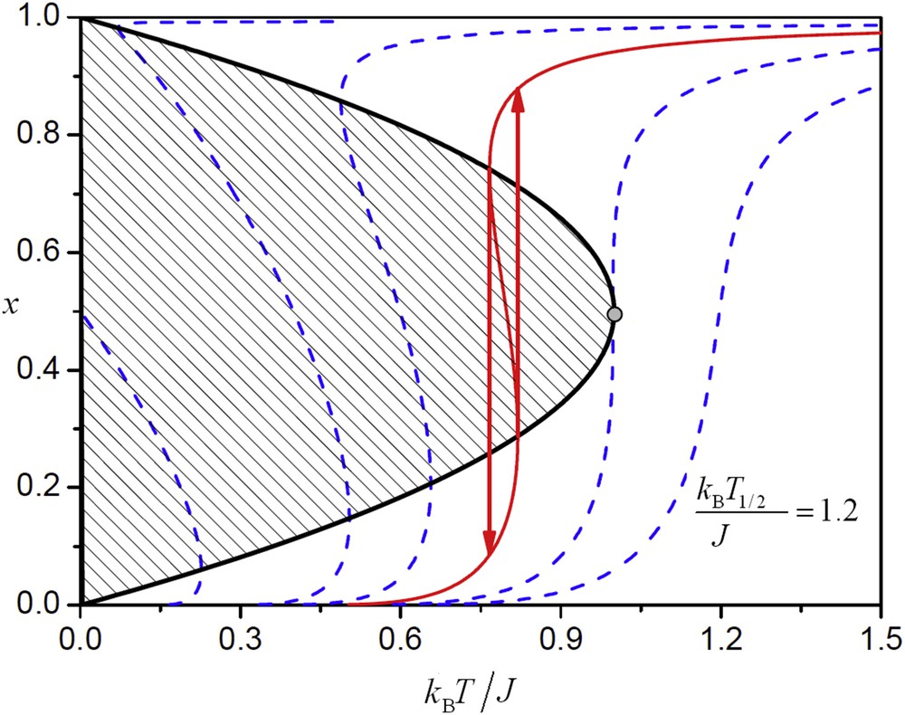
Relationship between the model parameters; the ratio critical for the presence of hysteresis is from left to right equal to 0, 0.4, 0.6, 0.8, 1.0 and 1.2, respectively. The shaded area is bordered by a spinodal curve where the HS and LS centres cannot coexist in a mixed state, i.e., the hysteresis appears. Adapted from Ref. [12].

A drawback of this simple model is the low flexibility of the shape of predicted transition curves.

To “translate” the presented microscopic parameters to experimentally attainable macroscopic quantities an alternative formulation of the model can be easily derived. If the SCO system is considered as a real solution (consistently with the presence of the cooperativity interaction) its molar Gibbs energy can be written in the form [13,14]

G = x G_{HS} + (1 - x) G_{LS} - T Δ S_{mix} + G_{int}

(8)

where

G_{HS}

and

G_{LS}

are partial molar Gibbs energies for individual SCO states,

G_{int}

is the excess interaction term accounting for the deviations from ideality of the solution and

Δ S_{mix}

is the mixing entropy. In the first approach, the approximate formula valid for ideal solutions can be used for mixing entropy

Δ S_{mix} \approx - R (x \ln x + (1 - x) \ln (1 - x))

(9)

The macroscopic counterpart of the mean-field cooperativity interaction is the Bragg–Williams (BW) approximation, which states for the interaction term

G_{int} \approx Δ_{BW} x - Γ_{BW} x^{2}

(10)

where Δ_BW and Γ_BW are parameters of the model that are often considered equal to each other. If thermodynamic equilibrium is reached at constant temperature and pressure, the system tends to attain composition at which Gibbs energy is minimal. Setting the derivative of Eq. 8 with respect to HS fraction equal to zero gives the following implicit equation:

x = \frac{1}{1 + \exp [\frac{Δ_{tr} H + Δ_{BW} - 2 Γ_{BW} x}{R T} - \frac{Δ_{tr} S}{R}]}

(11)

where all transition quantities of SCO are defined in a following manner

Δ_{tr} G = G_{HS} - G_{LS}

(12)

The transition enthalpy

Δ_{tr} H

and transition entropy

Δ_{tr} S

are related to transition Gibbs energy as

Δ_{tr} G = Δ_{tr} H - T Δ_{tr} S

(13)

The approach represented by Eq. 11 is called the thermodynamic model. Keeping Eq. 4 in mind, the comparison with Eq. 5 shows that Ising-like model within the MFA and thermodynamic model within the BW approximation are mathematically completely equivalent. Nevertheless, different point of view offers a useful physical insight; in this case the relationships between microscopic (Ising-like) and macroscopic (thermodynamic) parameters are obtained as follows [8]:

Δ = (Δ_{tr} H + Δ_{BW} - Γ_{BW}) / N_{A} \approx Δ_{tr} H / N_{A}

(14)

r = \exp (Δ_{tr} S / R)

(15)

J = Γ_{BW} / (2 N_{A})

(16)

The characteristic temperature derived from Eq. 6 results in the form

T_{1 / 2} = \frac{Δ_{tr} H + Δ_{BW} - Γ_{BW}}{Δ_{tr} S} \approx \frac{Δ_{tr} H}{Δ_{tr} S}

(17)

and the condition for the presence of hysteresis is given by

\frac{Δ_{tr} H}{Δ_{tr} S} < \frac{Γ_{BW}}{2 N_{A}}

(18)

3 Extensions of the basic model

One of the most popular improvements was motivated by analysis of the nature of the degeneracy ratio. It was shown that besides the simple ratio of spin multiplicity of HS and LS states (i.e., value of 3 for Fe(III) SCO systems and 6 for Fe(II) SCO systems), the inclusion of vibrational degree of freedom of SCO states is necessary to approach for the much higher experimental values [15]. For this sake, Bousseksou et al. considered the vibrations of the coordination environment and approximated them as independent harmonic oscillators. The form of Ising-like model is still preserved; however, novel effective quantities replace the original ones, namely [16]

r_{eff} = (\frac{g_{HS}^{el}}{g_{LS}^{el}}) \prod_{i = 1}^{3 n - 6} \frac{1 - \exp [- β h ν_{LS, i}]}{1 - \exp [- β h ν_{HS, i}]}

(19)

and

Δ_{eff} = Δ + (ε_{HS}^{vib} - ε_{LS}^{vib})

(20)

where n is the number of atoms in the relevant coordination environment (i.e., n = 6 for octahedron), ν_i are the frequencies of the normal vibration modes and ε^vib are the zero-point energies of the oscillators. If a mean frequency for each SCO state is introduced then the effective degeneracy ratio turns to

r_{eff} = (\frac{g_{HS}^{el}}{g_{LS}^{el}}) {(\frac{1 - \exp [- β h {\bar{ν}}_{LS}]}{1 - \exp [- β h {\bar{ν}}_{HS}]})}^{3 n - 6}

(21)

and if temperature is high enough (or, equivalently, if all vibration modes are considered equally populated) it collapses to

\lim_{T \to \infty} r_{eff} = (\frac{g_{HS}^{el}}{g_{LS}^{el}}) {(\frac{{\bar{ν}}_{LS}}{{\bar{ν}}_{HS}})}^{3 n - 6}

(22)

These adjustments provide elegant explanation for experimental values of transition entropy (related to parameter r) and allow coping with description of more gradual spin transitions than it was allowed by the original Ising-like model. Using this model the transition temperature has to be calculated iteratively

T_{1 / 2} = \frac{Δ_{eff}}{k_{B} \ln r_{eff} (T_{1 / 2})}

(23)

The hysteretic features of the Ising-like model can be improved by introduction of the distribution model as proposed by Boča and co-workers [7,17]. A large set of equidistant values of cooperativity parameter J₁, J₂, …, J_p is introduced and a weight factor is assigned to each of them. If the normal distribution is chosen the weight factor can be defined as

w_{i} = \frac{1}{δ \sqrt{2 π}} \exp [- {(J_{i} - \bar{J})}^{2} / 2 δ^{2}]

(24)

with mean value

\bar{J}

and a newly introduced parameter, the distribution variance δ. Corresponding set of average Ising spin values is obtained by using the implicit equation of the basic Ising-like model as discussed above, i.e.,

{〈 σ 〉}_{i} = - \tanh [β (Δ / 2 - J_{i} {〈 σ 〉}_{i}) - (\ln r) / 2]

(25)

and the overall average Ising spin is constructed with respect to the chosen distribution

〈 σ 〉 = \frac{\sum_{i = 1}^{p} w_{i} {〈 σ 〉}_{i}}{\sum_{i = 1}^{p} w_{i}}

(26)

Ideally, a fine grid shall be used (p → ∞) to avoid possible unphysical features of the model. In comparison with the basic Ising-like model, the parameter of cooperativity J is replaced here by the mean cooperativity $\bar{J}$ and one extra parameter (the distribution variance) appears. Obviously, for a very small value of variance the distribution model collapses to the original Ising-like model. Introduction of presented distribution manifests itself in the angling of the walls of the hysteresis loop—an experimentally observed feature that cannot be achieved within the genuine Ising-like model. Moreover, the wider the distribution variance, the stronger is the tendency to form incomplete transition (Fig. 2). The formula for transition temperature preserves the form given by Eq. 6 within this model.

Fig. 2
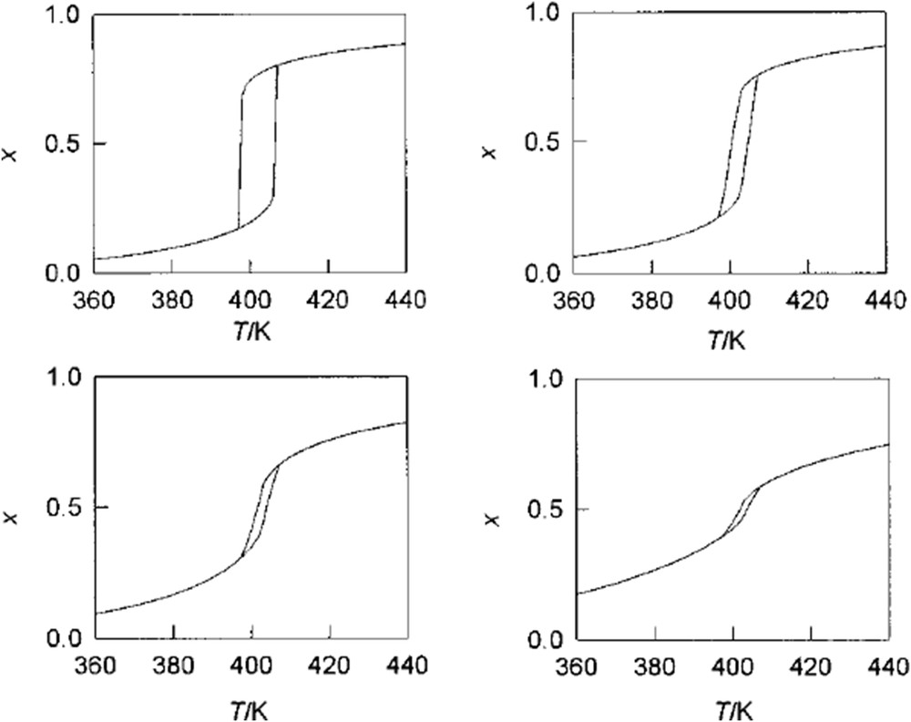
The effect of distribution of cooperativity on the SCO transition. The parameters were set as Δ = 2144 K, J = 452 K and r = 205, and the distribution variance equals to 10⁻⁵ (top left), 10⁻² (top right), 0.1 (bottom left) and 1.0 (bottom right). Adapted from Ref. [17].

The flexibility of the curve of transition can be significantly improved using the disorder model that was introduced by Chernyshov et al. [18]. A coupling of the SCO switching with a structural disorder (e.g., due to a lattice solvent) is supposed, leading to Hamiltonian in the form

{\hat{H}}_{i} = \frac{Δ}{2} {\hat{σ}}_{i} - J \sum_{j \neq i} {\hat{σ}}_{i} \cdot {\hat{σ}}_{j} + \frac{D}{2} {\hat{s}}_{i} - K \sum_{j \neq i} {\hat{s}}_{i} \cdot {\hat{s}}_{j} - I \sum_{j \neq i} {\hat{s}}_{i} \cdot {\hat{σ}}_{j}

(27)

where ŝ denotes the Ising spin associated with the disordered positions of a solvent. In its most complete form three novel parameters are introduced: D, K and I. The first two are counterparts of the Ising-like parameters Δ and J and the last one grasps the possible coupling of the Ising spins related to SCO and disorder. Within the MFA a system of two coupled implicit equations has to be solved iteratively:

〈 σ 〉 = - \tanh [β (Δ / 2 - J 〈 σ 〉 - I 〈 s 〉) - (\ln r) / 2]

(28)

〈 s 〉 = - \tanh [β (D / 2 - K 〈 s 〉 - I 〈 σ 〉)]

(29)

The transition temperature cannot be given explicitly; instead following implicit relation has to be obeyed [18]

T_{1 / 2} = \frac{Δ - 2 I 〈 s (T_{1 / 2}) 〉}{k_{B} \ln r}

(30)

The typical transition curves provided by this approach initially increase gradually and towards their completion ascend abruptly. The hysteresis loop tends to be centred above the transition temperature (Fig. 3).

Fig. 3
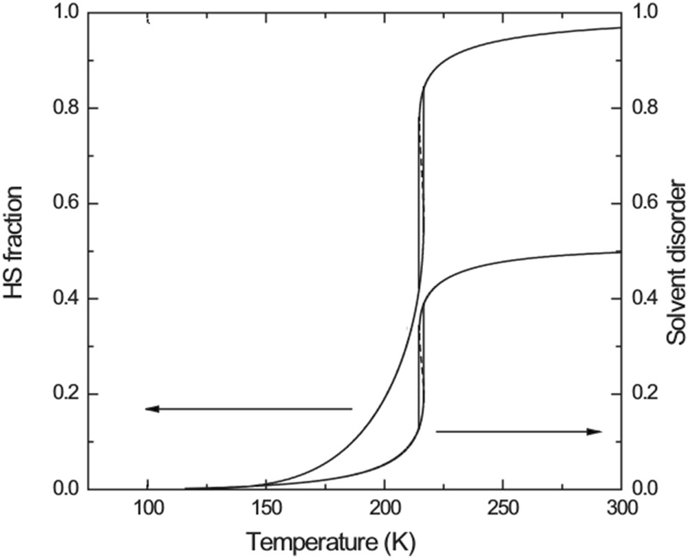
The effect of lattice solvent disorder coupled with SCO transition. The SCO parameters were set as Δ = 400 K, J = 20 K and r = 400, and the disorder parameters were set as D = 350 K, K = 0 K and I = 370 K. Adapted from Ref. [18].

The Ising-like model was also extended to encounter experimentally observed bi-step SCO transitions by Bousseksou and co-workers [19,20]. In order to achieve this, the model of two penetrating sublattices, A and B, with intralattice and interlattice cooperative coupling was postulated. Because bi-step transitions are often (but not necessarily) observed in binuclear systems, an intramolecular cooperativity can be introduced on top of the previous parameters. The complete Hamiltonian for the bi-step model within the MFA adopts the form

\hat{H} = \frac{Δ}{2} ({\hat{σ}}_{A} + {\hat{σ}}_{B}) + J_{1} ({\hat{σ}}_{A} 〈 {\hat{σ}}_{A} 〉 + {\hat{σ}}_{B} 〈 {\hat{σ}}_{B} 〉) + J_{2} ({\hat{σ}}_{A} 〈 {\hat{σ}}_{B} 〉 + {\hat{σ}}_{B} 〈 {\hat{σ}}_{A} 〉) + J_{A B} ({\hat{σ}}_{A} \cdot {\hat{σ}}_{B})

(31)

where J₁ is the cooperativity parameter acting between equivalent sites, J₂ the same between non-equivalent sites and J_AB quantifies the intramolecular cooperativity. To simplify its solution the symmetrically adapted quantities can be introduced as

\begin{array}{l} m = 〈 σ_{A} 〉 + 〈 σ_{B} 〉 \\ n = 〈 σ_{A} 〉 - 〈 σ_{B} 〉 \end{array}

(32)

and symmetrically adapted parameters as

\begin{array}{l} J_{+} = J_{1} + J_{2} \\ J_{-} = J_{1} - J_{2} \end{array}

(33)

The quantity m is proportional to the overall spin state value, whereas n indicates the breaking of symmetry in the SCO state between the sublattices. The system of two coupled implicit equations finally results

m = \frac{2 r^{2} \exp [- β (Δ + J_{+} m)] - 2 \exp [β (Δ + J_{+} m)]}{D}

n = \frac{- 4 r \sinh [β J_{-} n] \exp [2 β J_{AB}]}{D}

(34)

with the denominator

D = r^{2} \exp [- β (Δ + J_{+} m)] + \exp [β (Δ + J_{+} m)] + 2 r \exp [2 β J_{A B}] \cosh [β J_{-} n]

(35)

The model provides rich family of transition curves, with or without two steps and with the hysteresis loop present in the lower step or in both steps. For the case of symmetric binuclear systems a simplified version of the model is suitable where the two cooperativity parameters J₁ and J₂ are considered equal (if, furthermore, J_AB is omitted it collapses to the Ising-like model). Such an intervention excludes the presence of symmetry breakings (n = 0). Nevertheless, the ability to model the bi-step SCO transitions is preserved. The cost is only one extra parameter compared to the original Ising-like model [21]. The implicit equation for the mean Ising spin is then

〈 σ 〉 = \frac{r^{2} \exp [- β (Δ + 4 J 〈 σ 〉)] - \exp [β (Δ + 4 J 〈 σ 〉)]}{r^{2} \exp [- β (Δ + 4 J 〈 σ 〉)] + \exp [β (Δ + 4 J 〈 σ 〉)] + 2 r \exp [2 β J_{AB}]}

(36)

For this simplified version of a bi-step model for binuclear systems the transition temperature obeys again formula 6. However, the SCO state of a binuclear system is not uniquely characterized by T_1/2 because it is not necessarily formed by molecules in the intermediate molecular SCO state, i.e., LS–HS or HS–LS; some LS–LS and HS–HS pairs can occur at the transition temperature, as well. The maximum concentration of the intermediate state molecules can be used to define second characteristic temperature T_HL, which is within the simplified model given by [21]

T_{HL} = \frac{Δ}{k_{B} \ln r + k_{B} \ln \sqrt{\frac{Δ + 4 J_{AB}}{Δ - 4 J_{AB}}}}

(37)

Apparently, T_HL is equal to T_1/2 only if the intramolecular cooperativity is absent. The simplified bi-step model was also developed to cope with the possible presence of magnetic exchange interaction between the SCO centres in the HS–HS state [21]. Such an effect leads, in general, to smearing of the bi-step shape of the transition curve.

As already mentioned, the exact solution of Hamiltonian given by Eq. 2 for a special case with SCO particles arranged into chain can be derived exactly resulting in formula [9]

〈 σ 〉 = \frac{\sinh [β (Δ / 2) - (\ln r) / 2]}{{(\sinh^{2} [β (Δ / 2) - (\ln r) / 2] + \exp [- 4 β J])}^{1 / 2}}

(38)

Unlike the approximate solution given by Eq. 5, which does not take into account the geometry of the system, this exact solution predicts correctly that hysteresis cannot occur in a 1D cooperative system if the short-range interaction alone is present. Taking into account that by the SCO event the elastic strains can spread across the crystal inducing thus a long-range cooperative interaction, Linares et al. introduced an extra mean-field cooperative interaction to the basic model. The Hamiltonian of such a long-range Ising-like model possesses the form [9]

\hat{H} = \frac{Δ}{2} \sum_{i} {\hat{σ}}_{i} - J \sum_{i j} {\hat{σ}}_{i} {\hat{σ}}_{j} - G \sum_{i} {\hat{σ}}_{i} 〈 \hat{σ} 〉

(39)

where G is the parameter of the long-range cooperative interaction. Indeed, if solved within MFA, there is not any novelty brought to the basic Ising-like model (except that J is recast as J + G). The advantage is, however, that inclusion of the last term enriches the flexibility of the original model when preserving correct limiting behaviour. For instance, if long-range cooperativity is included into the exact solution of the Ising-like model for the 1D system, resulting implicit formula is already able to describe hysteretic behaviour and collapses to correct form for G → 0 [9]

〈 σ 〉 = \frac{\sinh [β (Δ / 2) - (\ln r) / 2]}{{(\sinh^{2} [β (Δ / 2 - G 〈 σ 〉) - (\ln r) / 2] + \exp [- 4 β J])}^{1 / 2}}

(40)

The incidence of physical stimuli during the temperature-induced SCO affects the thermal transition curve. It can be easily shown that if $(p_{i} E / k_{B} T) ≪ 1$ , with p_i being the electric dipole moment of a molecule in the respective SCO state and E the applied electric field, holds true, then the shift in the equilibrium temperature within limits of the basic Ising-like model is [22]

Δ T_{1 / 2} \approx \frac{(p_{HS}^{2} - p_{LS}^{2}) E^{2}}{2 k_{B} Δ}

(41)

Because usually p_HS > p_LS the electric field stabilizes the LS state and shifts the transition temperature to higher values. For a shift of 1 K the electric field of approximately 13 kV cm⁻¹ is necessary [23]. Similarly, if $(χ B / μ_{0} k_{B} T) ≪ 1$ is fulfilled, a simple estimation of the effect of magnetic field upon the SCO can be derived as [24]

Δ T_{1 / 2} \approx - \frac{(χ_{HS} - χ_{LS}) B^{2}}{2 μ_{0} k_{B} \ln r}

(42)

In contrast to the electric field, the HS state is favoured by the magnetic field as χ_HS > χ_LS. The decrease in transition temperature by 1 K is induced by magnetic field induction of approximately 22 T.

For the effect of pressure a simple macroscopic formula applies [10]

Δ T_{1 / 2} \approx \frac{p Δ_{tr} V}{Δ_{tr} S}

(43)

where Δ_trV stands for the difference in volume for the HS and LS phase. By insertion of typical values of the quantities, the formula predicts a shift by 1 K when the system is compressed by approximately 400 MPa.

Finally, let us emphasize that a rich class of vibronic models [25] and mechanoelastic simulations [2,26] were omitted in this article. Nevertheless, the interested reader should be able to get along with the basic principles and the vocabulary surveyed herein when studying a majority of the modern works on the SCO modelling.

4 Recent developments

Recent interest in SCO is mostly focused on the study of lithographic systems and nanoparticles [2,3]. Unlike the older models, which did not account for the size of studied systems, the behaviour of definite-sized SCO lattices appears to be dependent upon their precise dimension and shape [27]. Consequently, besides the Hamiltonian the lattice and boundary conditions also have to be specified. Usually the MFA is no more a satisfactory tool for their investigation and some more sophisticated techniques are to be adopted. Most popular ones are Monte-Carlo Metropolis (MCM) and Monte-Carlo Entropic Sampling (MCES). In simpler words, the MCM simulates the behaviour of interacting centres by random switching of their states. If the energy of new configuration is lower than the previous one, it is accepted, if it is higher, the rate of acceptance is given by the Boltzmann factor of the energy difference. By inspecting all sites of a system and repeating the step many times, the equilibrium value of any quantity can be calculated. This method was adapted for the SCO by Linares et al. who studied the basic Ising-like model [28] and the bi-step Ising-like model [29] for cubic lattices. Similarly to MCM, the nature of MCES lies in Monte-Carlo inspection of possible configurations; their occurrence is however biased, so that even the less probable configurations are accounted for. In this way, the degeneracy of each energy state is measured, and the partition function can be easily constructed from weighted Boltzmann factors. Having partition function determined, any desired quantity can be calculated. The MCES was adapted for needs of study of SCO phenomena by Shteto et al. [30] and Linares et al. [31] who researched the basic Ising-like Hamiltonian for 1D and 2D lattices. Besides the traditional transition curve, the methods based on the statistical physics can provide also the spatiotemporal picture of the transition, allowing thus the study of SCO phase nucleation and growth processes [2]. Discussion on such effects exceeds, however, the scope of the present work and interested reader is referred to specialized reviews in this journal.

Although the SCO behaviour upon reduction in size of the system is somehow inconclusive, the most often reported is the incompleteness of transition, the shifting down of transition temperature and narrowing or disappearance of hysteresis, which sometimes reappears at an ultrasmall scale [32]. Justified by the lower elastic strain felt by the surface sites, Muraoka et al. [33] fixed the permanent HS state for all peripheral SCO centres of an l × l square lattice and studied the basic Hamiltonian 2 (Fig. 4). For the simplest non-trivial sizes of this fixed-edge Ising-like model, the exact formula for Ising spin can be derived, namely, for l = 3 (i.e., one SCO active site) there holds true

〈 σ 〉 = \frac{8}{9} - \frac{1}{9} \tanh [β (Δ / 2 - 4 J) - (\ln r) / 2]

(44)

and for l = 4 (i.e., four SCO active sites) there results

〈 σ 〉 = \frac{3}{4} - \frac{1}{4} \frac{(\cosh [β (Δ / 2 - 2 J) - (\ln r) / 2] + \exp [- 2 β J]) \sinh [β (Δ / 2 - 2 J) - (\ln r) / 2]}{{(\cosh [β (Δ / 2 - 2 J) - (\ln r) / 2] + \exp [- 2 β J])}^{2} - 2 \exp [- 2 β J] \sinh^{2} [2 β J]}

(45)

Fig. 4
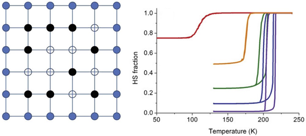
Square lattice with l = 6 illustrating the fixed-edge model. The blue edge centres are fixed in the HS state, whereas the central sites can acquire both, HS (black) or LS state (white, left picture). Calculated thermal dependence of the HS fraction for different sizes of the lattice; from left to right l = 4, 7, 10, 40, 200 (right picture). Adapted from Ref. [33].

The transition temperature is site-dependent and differs for centres neighbouring with two, one or none edge centre. In the first approach, the overall transition temperature can be derived as weighted average of the mentioned three values of T_1/2, resulting then in the following relationship:

T_{1 / 2} = \frac{Δ}{k_{B} \ln r} - \frac{8 J}{k_{B} \ln r} \frac{1}{l - 2}

(46)

The model offers a consistent prediction of the shift in the transition temperature to lower values for decreasing the nanoparticle size (Fig. 4). For large systems (l → ∞), Eq. 46 collapses to Eq. 6. The bigger lattices (l > 3) were studied using the MCM technique and showed that the main features of the experimental behaviour of SCO nanoparticles can be qualitatively reconstructed. As a less expected consequence of the model, a non-monotonous dependence of the width of the hysteresis loop upon the particle size was found.

Rather than imposing a particular SCO state, Enachescu and coworkers, Linares and coworkers and Boukheddaden and coworkers modelled in series of very recent works the effect of the surface by appending a matrix interaction term to the long-range Ising-like model for 1D [34], 2D [35–37] and 3D lattices [38–41]. The Hamiltonian was postulated as follows:

\hat{H} = \frac{Δ}{2} \sum_{i} {\hat{σ}}_{i} - J \sum_{i j} {\hat{σ}}_{i} {\hat{σ}}_{j} - G \sum_{i} {\hat{σ}}_{i} 〈 \hat{σ} 〉 - L \sum_{k} {\hat{σ}}_{k}

(47)

where L is the parameter of matrix interaction (the index k runs only over the surface centres). One can immediately see that the matrix interaction model collapses to the fixed-edge model when L diverges. Unlike the previous one, this model is too complicated to provide analytical solutions even for the smallest square lattices; this was studied by MCM and MCES methods. The model provides enormous varieties of multistep transitions with or without hysteresis loops [35]. Using similar arguments like those from the fixed-edge model the transition temperature can be estimated as [37]

T_{1 / 2} = \frac{Δ}{k_{B} \ln r} - \frac{8 L}{k_{B} \ln r} \frac{l - 1}{l^{2}}

(48)

This formula is equivalent to Eq. 46 when near-edge cooperativity L is set equal to the bulk cooperativity J and l includes edge sites. Choosing appropriate parameter values and MCES technique, it was demonstrated that in contrast to the long-range Ising-like model the matrix interaction model predicts appearance of hysteresis by decrease in the system size [36] (Fig. 5). This model was further studied for the case of ensemble of nanoparticles with distributed size [38–40].

Fig. 5
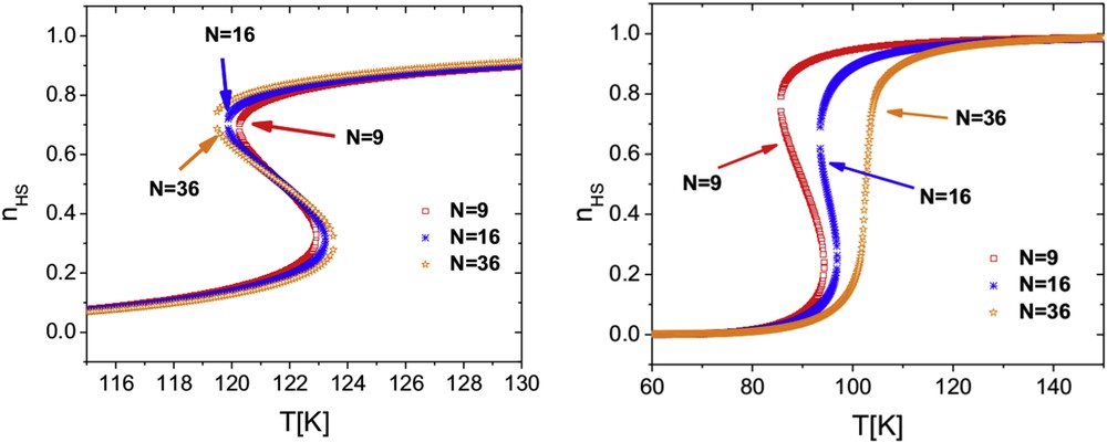
SCO in square nanoparticles of various sizes simulated by the long-range Ising-like model (left) and the matrix interaction Ising-like model (right). The common parameter values were set as Δ = 840 K, J = 10 K, G = 115 K and r = 992; for the latter L = 120 K. Adapted from Ref. [36].

Basic features of SCO in spherical nanoparticles can also be described with the non-extensive thermodynamic core–shell model within BW approximation. Félix et al.[42] defined the Gibbs energy of a nanoparticle as

G = x G_{HS} + (1 - x) G_{LS} - T (Δ S_{mix}^{b} + Δ S_{mix}^{s}) + S_{0} (x^{s} σ_{HS} + (1 - x^{s}) σ_{LS}) + Γ x (1 - x)

(49)

where superscripts s and b distinguish between surface and bulk quantities, respectively; S₀ stands for the unit-cell molar surface of the nanoparticle and σ_HS and σ_LS are the respective surface energies. It is convenient to also define the fractions of molecules on the surface and in the bulk, denoted as c^s and c^b, respectively. The overall HS fraction is then

x = c^{b} x^{b} + c^{s} x^{s}

(50)

In this model, different interaction constants, Γ_HS and Γ_LS, are considered for individual SCO states, which are related to the average parameter through

Γ = Γ_{LS} (1 - x) + Γ_{HS} x

(51)

Implying the concurrent condition of minimal Gibbs energy for surface and bulk, the following system of two coupled implicit equations results

x^{b} = \frac{1}{1 + \exp [\frac{Δ_{tr} H + Γ + (Γ_{HS} - Γ_{LS}) x (1 - x) - 2 Γ c^{b} x^{b} - 2 Γ c^{s} x^{s}}{R T} - \frac{Δ_{tr} S}{R}]}

(52)

x^{s} = \frac{1}{1 + \exp [\frac{Δ_{tr} H + Γ + (Γ_{HS} - Γ_{LS}) x (1 - x) - 2 Γ c^{b} x^{b} - 2 Γ c^{s} x^{s} + Δ (σ_{HS} - σ_{LS}) S_{0}}{R T} - \frac{Δ_{tr} S}{R}]}

(53)

A huge advantage of this approach is that the thermodynamic parameters are in principle measurable and often known. For example, the interaction terms are directly proportional to the bulk modulus of the material within the limits of BW approximation [43]. As apparent from Fig. 6, the total HS fraction evolves in qualitative accordance with expectation by decrease in the size. As shown by Mössbauer spectroscopy [42], the bulk modulus for ultrasmall nanoparticles is higher than that for the macroscopic systems. If this fact is taken into account, the reappearance of the hysteresis loop is predicted for nanoparticles. The transition temperature is derived as

T_{1 / 2} = \frac{Δ_{tr} H}{Δ_{tr} S} - \frac{Γ}{Δ_{tr} S} c^{s}

(54)

Fig. 6
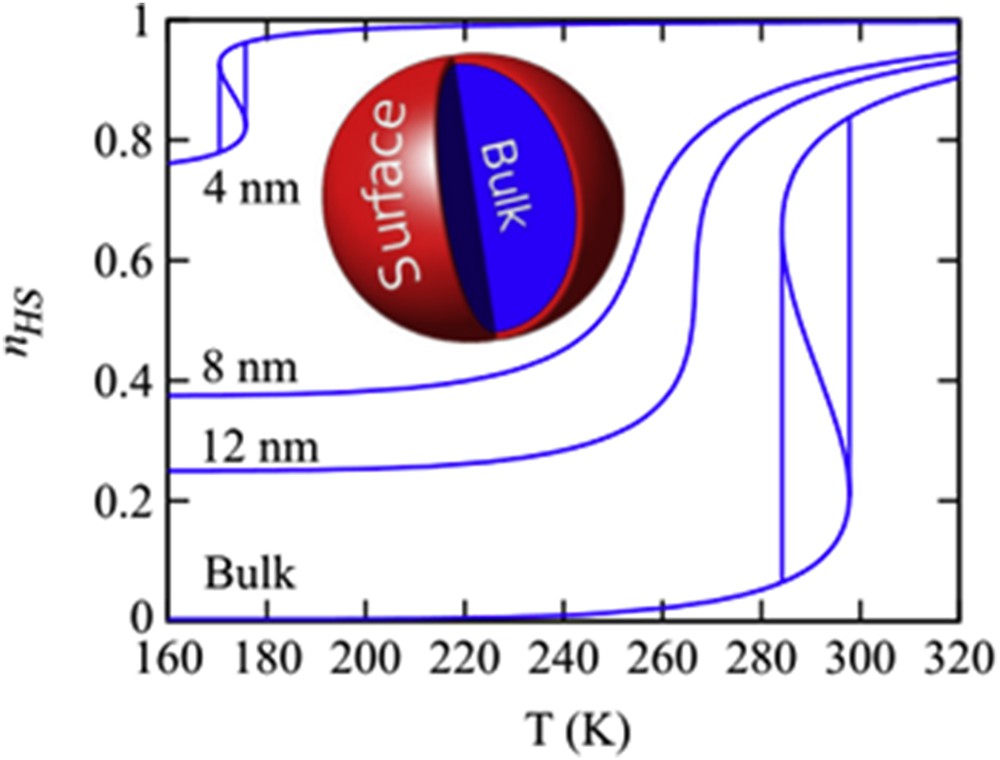
The effect of size of the spherical nanoparticle simulated by the non-extensive thermodynamic core–shell model where the SCO parameters were set as ΔH = 18 kJ mol⁻¹, ΔS = 61 J K⁻¹ mol⁻¹ and (σ_HS − σ_LS) = −0.1 J m⁻². For the 4 nm nanoparticle parameters were set as K_LS = 40 GPa and K_HS = 38 GPa; for the other sizes it applies K_LS = 24 GPa and K_HS = 18 GPa. Adapted from Ref. [42].

Again the transition temperature shifts down with increase in the fraction of particles forming the surface, i.e., by decrease in the radius of the sphere. For macroscopic systems it converges to Eq. 17 (Fig. 6).

Mikolasek et al. [44] solved Hamiltonian 2 in the local mean-field approximation (LMFA). The key idea behind this technique is averaging of Ising spins of only those centres that directly neighbour to interrogated centre, rather than averaging over the entire system. The solution of Hamiltonian 2 leads to following coupled system of implicit equations:

〈 σ_{i} 〉 = - \tanh [β (Δ / 2 - J M_{i}) - (\ln r) / 2]

(55)

where

〈 σ_{i} 〉

is the thermodynamic average of Ising spin of ith site and the quantity M_i is the local mean field at this site defined as

M_{i} = \frac{1}{q_{i}} \sum_{j}^{q_{i}} 〈 σ_{j} 〉

(56)

where j runs over the q_i neighbours of site i. To mimic a cubic system with primitive packing of molecules, q_i was set equal to 6 in the core, whereas at the surface, edges and corners, it was set equal to 5, 4 and 3, respectively. Furthermore, for the surface sites the degeneracy ratio was enhanced. The LMFA Ising-like model predicts decrease in transition temperature and hysteresis width with decrease in the size of the cube, eventually turning to smooth incomplete transition when the level of nanoparticles is reached (Fig. 7).

Fig. 7
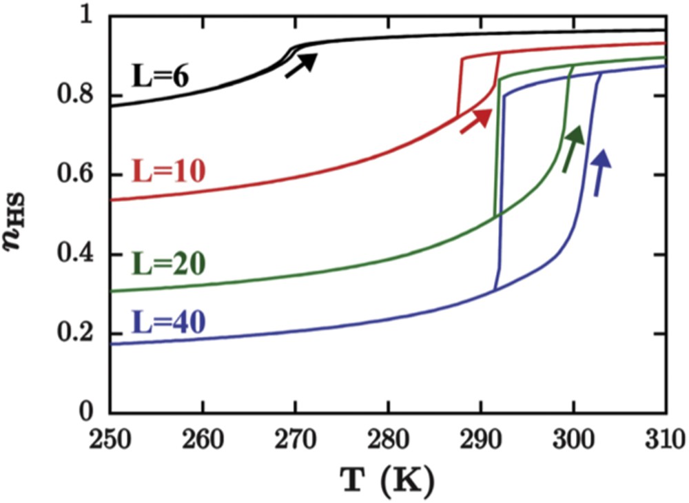
The size effect for the cubic SCO nanoparticle simulated by the LMFA Ising-like model. The parameters were set as Δ = 1220 K, J = 60 K and r = 63 for the core sites when r = 6568 for the surface sites. Adapted from Ref. [44].

5 Conclusions

Various models on the temperature-induced SCO transitions have been reviewed with the focus on simplicity. It has been shown that the phenomena like hysteresis and bi-step transitions can be in the simplest cases satisfactorily modelled with three empirical parameters. In the more elaborated models the effect of vibrations, effect of crystal solvents, multistep transition or size extensiveness are included extending thus significantly the range of their applicability. The basic features of temperature-induced SCO in nanoparticles are successfully grasped within the frame founded by the Ising-like model and its derivatives.

To sum up, the Ising-like model and its derivatives form a very handy working tool for exploration of SCO-related phenomena and even sophisticated interpretations of macroscopic SCO behaviours keep the vocabulary introduced by them.

Acknowledgements

Slovak grants APVV-14-0073, APVV-14-0078, VEGA 1/0125/18, KEGA 017STU-4/2017 and STU Grant Scheme for Support of Excellent Teams of Young Researchers (BIOKA 1664) and the French Ministry of Higher Education, Research and Innovation, University of Versailles, CNRS (UMR N° 8635) and grant ANR BISTA-MAT, ANR-12-BS07-0030-01, are highly appreciated for financial support.

Bibliographie

[1] Spin Crossover: Properties and Applications (M.A. Halcrow, ed.), Wiley-VCH, Weinheim, 2013

[2] A. Boussesksou; G. Molnár; L. Salmon; W. Nicolazzi Chem. Soc. Rev., 40 (2011), pp. 3313-3335

[3] K.S. Kumar; M. Ruben Coord. Chem. Rev., 346 (2017), pp. 176-205

[4] J. Wajnflasz Phys. Stat. Sol., 40 (1970), pp. 537-545

[5] J. Wajnflasz; R. Pick J. Phys. Colloq., 32 (1971), pp. 90-91

[6] E. König Struct. Bond., 76 (1991), pp. 51-152

[7] R. Boča; W. Linert Monatsh. Chem., 134 (2003), pp. 199-216

[8] J. Pavlik; R. Boča Eur. J. Inorg. Chem. (2013), pp. 697-709

[9] J. Linares; H. Spiering; F. Varret Eur. Phys. J. B, 10 (1999), pp. 271-275

[10] F. Varret; S.A. Salunke; K. Boukheddaden; A. Bousseksou; E. Codjovi; C. Enachescu; J. Linares C. R. Chimie, 6 (2003), pp. 385-393

[11] J.P. Tuchagues; A. Bousseksou; G. Molnár; J. McGarvey; F. Varret Top. Curr. Chem., 235 (2004), p. 85

[12] K. Boukheddaden; I. Shteto; B. Hôo; F. Varret Phys. Rev. B, 62 (2000), pp. 14796-14805

[13] C.P. Slichter; H.G. Drickamer J. Chem. Phys., 56 (1972), pp. 2142-2160

[14] P.S. Rao; P. Ganguli; B.R. McGarvey Inorg. Chem., 20 (1981), pp. 3682-3688

[15] M. Sorai; S. Seki J. Phys. Chem. Solids, 35 (1974), pp. 555-570

[16] A. Bousseksou; H. Constant-Machado; F. Varret J. Phys. I France, 5 (1995), pp. 747-760

[17] R. Boča; M. Boča; Ľ. Dlháň; K. Falk; H. Fuess; W. Haase; R. Jaroščiak; B. Papánková; F. Renz; M. Vrbová; R. Werner Inorg. Chem., 40 (2001), pp. 3025-3033

[18] D. Chernyshov; N. Klinduhov; K.W. Törnroos; M. Hostettler; B. Vangdal; H.B. Bürgi Phys. Rev. B, 76 (2007), p. 014406

[19] A. Bousseksou; J. Nasser; J. Linares; K. Boukheddaden; F. Varret J. Phys. I France, 2 (1992), pp. 1381-1403

[20] A. Bousseksou; F. Varret; J. Nasser J. Phys. I France, 3 (1993), pp. 1463-1473

[21] J. Pavlik; W. Nicolazzi; G. Molnár; R. Boča; A. Bousseksou Eur. Phys. J. B, 86 (2013), p. 292

[22] T. Mahfoud; G. Molnár; S. Bonhommeau; S. Cobo; L. Salmon; P. Demont; H. Tokoro; S. Ohkoshi; K. Boukheddaden; A. Bouseksou J. Am. Chem. Soc., 131 (2009), p. 15049

[23] C. Lefter; R. Tan; J. Dugay; S. Tricard; G. Molnár; L. Salmon; J. Carrey; W. Nicolazzi; A. Rotaru; A. Bousseksou Chem. Phys. Lett., 644 (2016), p. 138

[24] A. Bousseksou; F. Varret; M. Goiran; K. Boukheddaden; J.-P. Tuchagues Top. Curr. Chem., 235 (2004), p. 62

[25] M. Dimian; A. Rotaru Magnetic Materials (K. Maaz, ed.), Intech Open Limited, London, 2016

[26] L. Stoleriu; P. Chakraborty; A. Hauser; A. Stancu; C. Enachescu Phys. Rev. B, 84 (2011), p. 134102

[27] T. Kawamoto; S. Abe Chem. Commun. (2005), pp. 3933-3935

[28] J. Linares; J. Nasser; K. Boukheddaden; A. Bousseksou; F. Varret J. Mag. Mag. Mater., 140–144 (1995), pp. 1507-1508

[29] J. Linares; J. Nasser; A. Bousseksou; K. Boukheddaden; F. Varret J. Mag. Mag. Mater., 140–144 (1995), pp. 1503-1504

[30] I. Shteto; J. Linares; F. Varret Phys. Rev. E, 56 (1997), p. 5128

[31] J. Linares; C. Enachescu; K. Boukheddaden; F. Varret Polyhedron, 22 (2003), pp. 2453-2456

[32] M. Mikolasek; G. Félix; W. Nicolazzi; G. Molnár; L. Salmon; A. Bousseksou New J. Chem., 38 (2014), pp. 1834-1839

[33] A. Muraoka; K. Boukheddaden; J. Linares; F. Varret Phys. Rev. B, 84 (2011), p. 054119

[34] D. Chiruta; C.-M. Jureschi; J. Linares; P.R. Dahoo; Y. Garcia; A. Rotaru Eur. Phys. J. B, 88 (2015), p. 223

[35] C.-M. Jureschi; B.-L. Pottier; J. Linares; P.R. Dahoo; Y. Alayli; A. Rotaru Physica B, 486 (2016), pp. 160-163

[36] J. Linares; C.M. Jureschi; A. Boulmaali; K. Boukheddaden Physica B, 486 (2016), pp. 164-168

[37] J. Linares; C.M. Jureschi; K. Boukheddaden Magnetochemistry, 2 (2016), p. 24

[38] A. Atitoaie; R. Tanasa; C. Enachescu J. Mag. Mag. Mater., 324 (2012), pp. 1596-1600

[39] A. Atitoaie; R. Tanasa; A. Stancu; C. Enachescu J. Mag. Mag. Mater., 368 (2014), pp. 12-18

[40] A. Atitoaie; L. Stoleriu; R. Tanasa; A. Stancu; C. Enachescu Physica B, 486 (2016), pp. 138-141

[41] C.M. Jureschi; J. Linares; A. Rotaru; Y. Garcia Magnetochemistry, 2 (2016), p. 13

[42] G. Félix; W. Nicolazzi; L. Salmon; G. Molnár; M. Perrier; G. Maurin; J. Larionova; J. Long; Y. Guari; A. Bousseksou Phys. Rev. Lett., 110 (2013), p. 235701

[43] H. Spiering; K. Boukheddaden; J. Linares; F. Varret Phys. Rev. B, 70 (2004), p. 184106

[44] M. Mikolasek; W. Nicolazzi; F. Terki; G. Molnár; A. Bousseksou Phys. Chem. Chem. Phys., 19 (2017), p. 12276