A perturbation method to estimate building thermal performance

Florent Alzetto; Johann Meulemans; Guillaume Pandraud; Didier Roux

doi:10.1016/j.crci.2018.09.003

Résumé

The Quick U-Building (QUB) method is a dynamic method developed to estimate the heat loss coefficient of a building in one night without occupancy. Feasibility measurements and comparisons with various references have been done in earlier studies whatever numerically, experimentally in an ideal case, or experimentally in real cases. This article presents a review of various perturbation methods developed to assess building thermal performance, details of theoretical understanding of the QUB method, and gathers experimental results obtained in many different configurations. The heat loss coefficients estimated with the QUB method are in good agreement with experimental references and are reproducible. This demonstrates that the QUB method has a real potential to estimate the heat loss coefficient of a building in a short duration and with a reasonable accuracy.

1 Introduction

In the second half of the last century, perturbation methods have been developed to obtain thermodynamical constants of chemical reactions [1]. These methods have been widely used to become a classical tool to these.

Thermal performance of a building is extensively calculated but very rarely measurements are implemented. A building can be considered as a thermodynamical body whose equilibrium among internal temperature, external temperature, and energy needed to maintain a difference in temperature is linked by a differential equation with two series of constants: heat capacities of the materials and thermal leakages due to the thermal conductivity of the very same materials and air infiltrations. A simplified version of the system can be described using averaged values of these parameters [2] and includes an apparent thermal capacitance and the building heat loss coefficient. The characteristic time is given by the ratio of this capacity and the heat loss coefficient. Measuring thermal performances of a building is more complex because usually this characteristic time is of the order of several days meaning that a building is never in a steady state, which would be the easiest way to measure the building thermal resistance. It is in this specific technical context that the idea of using perturbation methods to access the thermal parameters of a building is born.

In this article, we first propose a review of existing methodologies to estimate building thermal performance. Then we detail the theoretical understanding developed on the Quick U-Building (QUB) method and a criterion that is considered for a measurement. Finally, we gather measurements performed in many different configurations and show that the results are in good agreement with references and reproducible.

2 Methods to measure the thermal performance of buildings

To estimate building thermal properties, we distinguish three different categories of methodologies. All consists in monitoring various physical quantities such as temperatures, heat fluxes, climatic data, or power consumption. In addition, a thermal model is defined to describe relation between these physical properties as a function of a set of parameters. These parameters can represent a heat loss coefficient, a solar aperture, or a thermal inertia and are identified using inverse techniques by minimizing residuals between the monitored data and the predicted ones from the model.

A first category is composed of quasi-static methodologies. In 1979, one of the first methodologies using this approach developed by the Lawrence Berkely National Laboratory is the coheating technique [3]. It consists in regulating the building with electrical heaters at a given temperature during the cold season. Inside and outside temperatures as well as electrical consumptions are monitored during a few weeks (usually 2–4 weeks depending on the climatic conditions). The model is a static relation between the measured parameters and the physical properties identified. These are the heat loss coefficient and the solar aperture. It describes the heating needs (electrical consumption) to compensate heat losses (function of the temperature difference) minus the solar heat gains (function of global horizontal solar irradiance). As the inside temperature is regulated, only the external conditions and so heating needs vary in time. A quasi-static approach is therefore used by averaging on a daily basis the physical quantities monitored. More recently a methodology based on this technique has been formalized in 2013 by Leeds Beckett University [4] and a review article has been published [5].

A second category is composed of dynamic methodologies, which consists in performing a well-defined heat load. These are perturbation-based methods. In 1988, the Primary and Secondary Terms Analysis and Renormalization (PSTAR) methodology has been proposed by the Solar Energy Research Institute [6]. The recommended heat load is composed of a temperature regulation phase followed by a free-cooling phase during cold season. Various physical quantities can be monitored and their selection is based on a preliminary building audit. In 2012, a methodology called QUB [2] has been proposed. It consists in a dynamical heat load using electrical heaters, which is composed of a constant-heating phase of a few hours followed by a free-cooling phase of the same duration. This shall be done at night without occupancy. Inside and outside temperatures and electrical power consumption are monitored. Heat loss coefficient and an apparent thermal capacitance are estimated. In 2014, the In Situ Assessment of Building EnveLope performancEs (ISABELE) methodology [7] has been proposed. The thermal heat load is done in three phases without occupancy and in cold season. The first phase consists in a temperature increase using a constant heating power for about 24 h. This is followed by a temperature regulation phase for few days and finally a free-cooling period of about 24 h. Inside temperature, electrical power consumption, and climatic data are monitored. Heat loss coefficient and an apparent thermal capacitance are identified.

The third category is composed of dynamic methodologies but assuming that the building may be occupied. It means that contrarily to the previously described category of methods, no heat load is specifically designed and these often require additional physical measurements and the use of more complex models. Complex models associated with inverse techniques are used to identify building characteristics. In 2006, Ghiaus [8] proposed a methodology to assess building energy performance based on a simple monitoring. In 2011, Mejri et al. [9] proposed modeling toolbox to describe building dynamics and so to estimate by inverse technique physical parameters. In the next section, we focus on the QUB method and its theoretical understanding to explain how it should be used to estimate building thermal performance.

3 Theoretical understanding of the QUB method

The QUB methodology is based on a one-time constant model [2]. Using the electrical–thermal analogy [10], it consists in separating the inside and the outside temperature nodes by a thermal resistance representing the heat loss of the building envelope. In addition, a thermal capacitance and a thermal source are located at the inside temperature node (see Fig. 1)..

Fig. 1
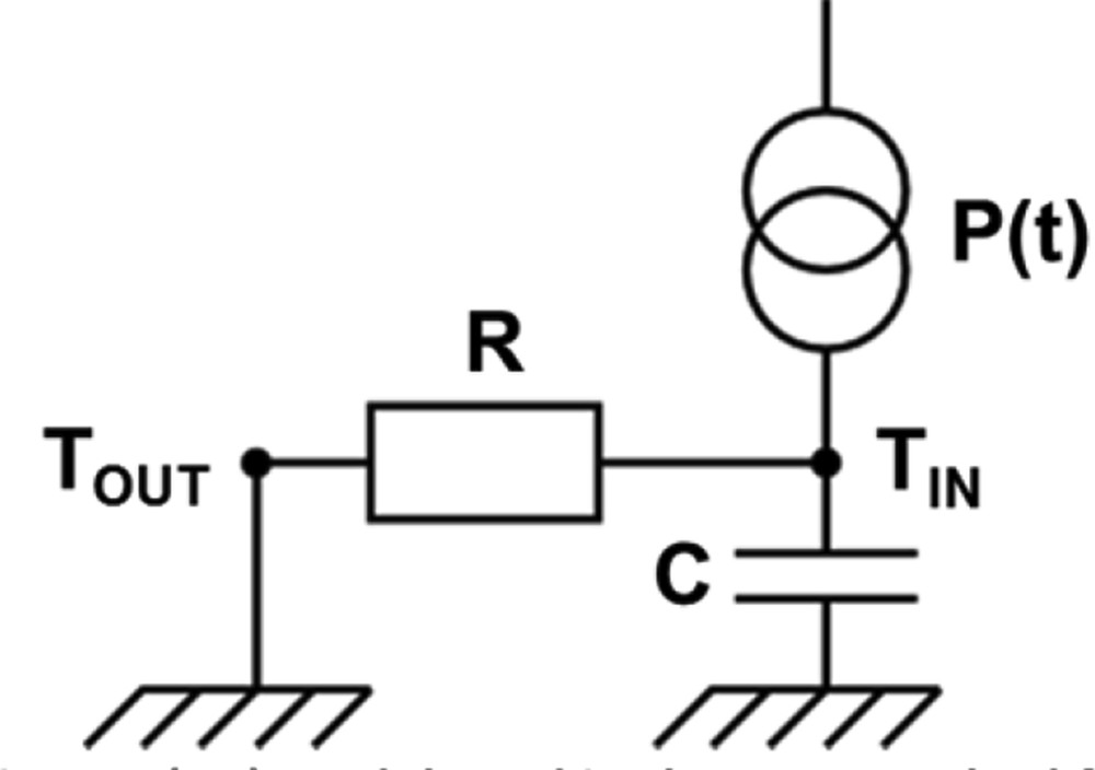
The resistance–capacitance (RC) model used in the QUB method for assessing the Host Language Call (HLC) of buildings.

These describe a thermal mass, which can be heated using a heater inside the building. This dynamical model is intended to describe thermal losses through the building envelope and thermal storage within the building fabric. The two unknown physical parameters are a thermal resistance (its inverse is H in Watt per Kelvin) and a thermal capacitance (noted C in Joule per Kelvin). In this simplest case, the dynamic relation between parameters is given by Eq. 1 (thermal balance of the simplest equivalent building model) Ref. [2]:

C d T = (P - H Δ T) d t

(1)

where

P

the inside thermal power brought by all heating sources inside of the house and possibly the solar gain and

Δ T

is the difference between the inside and outside of air temperature. This methodology was primarily designed to work at night using electrical heaters and without occupancy. This was to accurately measure the heating power transmitted to the inside temperature node. The heat load is composed of two distinct phases (see Fig. 2), a constant-heating-power phase followed by a free-cooling phase. Both phases last for the same duration so that the entire test fits within a night.

Fig. 2
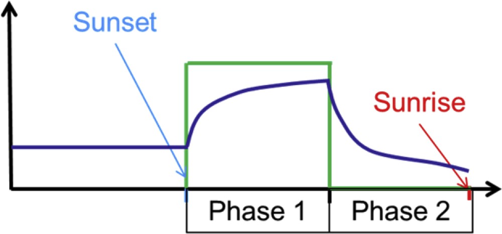
Schematic of heating power and temperature evolution during the two consecutive phases.

The model inversion is only performed using the data set at the end of each phase (a few hours for a long enough experiment). It means that the transitory regime is not taken into account for physical parameter identification. Theoretically the thermal response of a one-dimensional assembly of homogeneous layers in series to this heat load would be an infinite summation of time-decay exponentials [11,12]. Therefore, by performing a long-enough constant heat load, only one time constant would still have a non-negligible contribution and therefore the model would be valid (see Eq. 2, i.e. the general form of the temperature response to a constant heat load and its limit at long time).

Δ T (t) = \frac{P}{H} + [Δ T (t_{0}) - \frac{P}{H}] \sum_{i} a_{i} e^{- t / τ_{i}} \underset{t ≫ τ_{n - 1}}{\to} \frac{P}{H} + [Δ T (t_{0}) - \frac{P}{H}] a_{n} e^{- t / τ_{n}}

(2)

where

t_{0}

is the time at which the heat load is submitted,

τ_{i}

are time constants (it will be assumed here that they have an increasing value from

τ_{1}

, the smallest time constant, to

τ_{n}

, the largest), and

a_{i}

are constants depending on model resistances, capacitances, and on initial conditions.

To go further, a quadrupole model has been used to describe the experiment [12]. It exactly describes in the state space the temperature response during the experiment with a static initial condition. Using the assumption that the temperature response is an infinite summation of time-decay exponentials, it has been shown that the heat loss coefficient estimated using the QUB method is exactly equal to the building heat loss coefficient for specific conditions only. There is a bias that depends on the heating power and on the heating duration. The error is nil when the heating duration is large enough (as compared with the building time constants) and when the heating power is finite such as the inside temperature remains constant. This model shows that the error increases with a dimensionless parameter $α = (P - H Δ T_{0}) / P$ and decreases with the heating duration. To get a more realistic simulation we may precede the experiment by a free-cooling phase to get a dynamical initial condition. In this case, we show that the heat loss estimated is lower than it would have been with a static initial state but the main dependence remains similar (Fig. 3).

Fig. 3
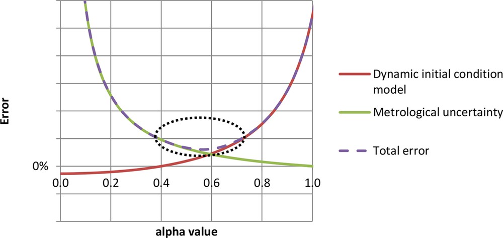
Schematic representation of main error sources as a function of α. The red solid line is the model error, the green solid line is the metrological uncertainty, and the dashed purple line is the total error (quadratic sum of the two error sources).

Finally, an excessively low heating power (i.e. close to, or lower than, the heating power needed to maintain the temperature constant and equal to its initial value, which corresponds to $α \to 0$ ) or an excessively small heating duration will result in very low temperature variations and so to a relatively higher metrological uncertainty on the estimated heat loss coefficient. On the contrary, a very high heating power (i.e. $α \to 1$ ) will reduce metrological uncertainty (Fig. 3).

From this understanding there exists a range of values of α for which the model error and the metrological uncertainty are optimal to minimize the total error on the estimated heat loss coefficient. This has led to the power criterion, which recommends to perform measurement with 0.4 < α < 0.7 (Fig. 3). Anyway we have to mention that the increase in the heating duration will reduce both error sources (model bias and metrological uncertainty). In the next section, we demonstrate the feasibility of this method in an ideal case following this power criterion.

4 Experimental demonstration on an ideal case

To experimentally demonstrate the feasibility of the QUB method, measurements have been performed in an ideal case [13], a typical full-scale UK building, which is located in a climate chamber (it means that the temperature of the external environment can be controlled for several days and that there is no direct solar radiation). The main advantage is that we are able to perform a direct and reliable measurement of the building heat loss coefficient. It requires to maintain the temperature to a given set point using a regulator and to wait for several days to reach a steady state. The building heat loss coefficient is therefore the ratio of the heating power and the difference in inside–outside temperature.

The building has been retrofitted using five different retrofit materials, and at each stage a static and a QUB measurement (4 h heating duration, except for stage 2 where heating duration was 30 min) has been performed [13]. Retrofit stages include windows replacement, loft insulation, suspended timber floor insulation, and internal wall and external wall insulation to cover a wide range of construction details. In the various tests, the maximum deviation between static and QUB measurement is 15%, which demonstrates the possibility to use the QUB method to assess the building heat loss coefficient in a short duration with an acceptable accuracy.

In a second phase, additional measurements of building thermal performance have been carried out in two cases, a nonretrofitted one and a fully retrofitted one using high-performance windows and internal wall insulation [14,15]. In the various tests performed, the influence of the heating power and the heating duration has been tested. The behavior expected by the theoretical approach (Fig. 3) has been observed experimentally. It has been shown in these two cases, by performing a long enough measurement (4 h heating duration), a very good reproducibility and a maximum deviation of 10% could be reached. Very short measurements have been experimented (30 min and 1 h) and a larger deviation has been observed (less than 40% difference as compared with the reference). A summary of the tests performed is provided in Table 1.

Table 1

Stage [Reference article]	Insulation	Thermal inertia	Reference	QUB
Number of tests	HLC (W/K)	Uncertainty (%)	Standard deviation with 95% confidence interval (%)	Deviation from reference (%)
1 [13]	Yes	Average	70 ± 3	1	77	11	NA	10
2 [13]	Almost total	Average	83 ± 3	1	95	7	NA	15
3 [13]	Almost total	Average	101 ± 3	1	116	7	NA	15
4 [13]	Only glazing	Average	174 ± 4	1	198	5	NA	14
5 [13]	Only loft	Average	181 ± 4	1	198	6	NA	10
6 [13]	No	Average	188 ± 4	1	212	6	NA	13
7 [14,15]	No	Average	240 ± 10	14	213	NA	6	−12
8 [14,15]	Yes	Low	59 ± 2	4	60	NA	12	2

We observe first, for all of the insulation and thermal inertia levels tested, a very good agreement with the reference value (the maximum deviation is 15%). Second, for measurements where several tests have been performed, we observe a very good reproducibility of the measurements (standard deviation with 95% confidence interval is at most 12%). This shows that in this controlled case the QUB method is reproducible and able to provide the correct estimation of the heat loss coefficient in less that one night.

These experiments have a limitation, which is the absence of realistic climatic conditions on the building. It lacks solar radiation, external temperature variations, and wind influence. For these purposes several measurements have been done in the field. In the next section, we demonstrate, for real cases, the good reproducibility and the good agreement with various experimental methodologies.

5 Real cases application of the QUB method

After the initial experiment done in a house of the south of France [2], another series of measurements in the field have been done in an internally well-insulated two-storey single-family house of 131 m² floor area, located in France. Six measurements have been done in winter and in summer (24 h heating duration) [11]. Even if the average of the results obtained is higher than the calculated estimation we observe a very good reproducibility, whether the measurements have been done in winter or in summer. The standard deviation with 95% confidence interval is around 10% of the average value. Even if we cannot conclude on the absolute value of the heat loss coefficient, this demonstrates that the QUB method is able to provide reproducible and consistent results on new built, whatever the outside conditions.

A second series of measurements have been done in a hybrid and well-insulated two-storey single-family house of 88 m² floor area in France. Seven measurements were performed in winter (heating duration, 7 h) and an experimental comparison with ISABELE methodology has been done, in addition to a detailed thermal study [7]. The average of the results is in very good agreement with the thermal study (6% of deviation) and with the ISABELE measurement (12% of deviation). The standard deviation with 95% confidence interval, based on six tests, is around 20% of the averaged value. So this shows again that even in real conditions, the QUB method can provide reproducible and consistent measurements on new built.

Another experimental campaign has been performed in an externally well-insulated two-storey single-family house of 164 m² floor area. Ten QUB measurements were performed in winter condition (heating duration, 4 h and 30 min) and a comparison measurement using the coheating methodology [4] has been done in addition to a detailed thermal study [12]. QUB measurements have been done according to the power criterion. The average of the 10 measurements is in very good agreement with the thermal study (4% of deviation) and with the coheating measurement (5% of deviation). The standard deviation with 95% confidence interval is around 13% of the average value. This case also demonstrates that the QUB method provides results consistent with another experimental method and is reproducible even on new built with external wall insulation.

A last experimental campaign has been done in a noninsulated two-storey single-family house with a 186 m² floor area in the UK. Two air permeability levels have been investigated. In these low- and high-airtightness levels, 52 and 94 QUB measurements in winter conditions were, respectively, performed (between 5 and 7 h of heating duration) [16]. QUB measurements have been done following the power criterion. In both cases, averages are close and consistent with the air permeability level, meaning that the higher the air permeability, the higher the heat loss coefficient. Standard deviations with 95% confidence interval are, respectively, 15% and 18%. This case demonstrates once again that the QUB method is able to provide consistent and reproducible results. A summary of all the experimental results obtained is provided in Table 2.

Table 2

Reference article	Insulation	Thermal inertia	Reference	QUB
Method	H in W/K	Heating duration	Number of tests	H in W/K	Standard deviation with 95% confidence interval (%)	Deviation from reference (%)
[11]	Yes	Low	Thermal study	100	12 h	6	133	9	33
[7]	Yes	Average	Thermal study	105	7 h	6	99	20	6
ISABELE	112	12
[12]	Yes	High	Thermal study	119	4.5 h	10	115	13	4
Coheating	121	5
[16]	No	Average	NA	NA	5–7 h	52	522	15	NA
No	Average	NA	NA	5–7 h	94	508	18	NA

We observe first that even in the field and for all of the thermal insulation and inertia levels, results are very reproducible. The maximum standard deviation with 95% confidence interval is 20%. Second, the absolute value estimated is very close to reference experimental measurements (i.e. ISABELE or coheating, not thermal studies). The largest deviation is 12% from the reference. Comparing with thermal studies, we observe a larger difference, which could be because of the uncertainty of the calculation method or a performance gap. These experiments demonstrate that even in real field and for very different thermal insulation and inertia levels, this method is reproducible and provides a heat loss coefficient estimation very close to the experimental reference. This indicates a huge potential toward building envelope quality assessment in the field.

6 Conclusions

We see that perturbation methods, as the one that has been developed to study the kinetics of chemical reaction, can be used for measuring the thermal performance of a building. The main advantages of this method are its simplicity and duration, and therefore its potential cost. In only a few hours, one can obtain in a reliable way the total heat loss coefficient of the building. This method has been tested in models as well as real buildings and gives good results in a very consistent fashion.

Acknowledgments

The authors thank all of the contributors to the experimental works discussed in this article: V. Sougkakis, D. Gossard (Saint-Gobain), D. Farmer (Leeds Metropolitan University), R. Fitton (University of Salford), I. Heusler (Fraunhofer IBP), R. Bouchié and S. Thébault (CSTB), and A. Brun (CEA). The authors also thank Saint-Gobain for funding.