


 CC-BY 4.0
1. Introduction
In addition to the precise theoretical and experimental description of X-ray fluorescence (XRF) spectroscopy previously made [1, 2, 3, 4, 5, 6, 7], the present review is nonetheless important in order to show the clinician the kind of sample that can be investigated using XRF, the kind of information that can be derived from these analyses and how it competes with other analytical tools [8, 9, 10, 11, 12, 13].
Methods for trace element analysis
| Analytical methods | |
|---|---|
| Destructive analysis | AAS (atomic absorption spectroscopy) |
| ICP-AES (inductively coupled plasma-atomic emission spectroscopy) | |
| ICP-MS (inductively coupled plasma-mass spectroscopy) | |
| Semi-destructive | LA-ICP-MS (laser abrasion-ICP-MS) |
| SIMS (secondary ion mass spectroscopy) | |
| Non-destructive | EDS (energy dispersive X-ray spectroscopy) or WDS (wavelength dispersive X-ray spectroscopy) |
| XRF | |
| NAA (neutron activation analysis) | |
| PIXE (particle induced X-ray emission spectroscopy) | |
For example, while vibrational spectroscopies such as Infrared spectroscopy used routinely at the hospital [14, 15, 16] give accurate determination of the chemical composition of kidney stones, these vibrational techniques are unable to assess the presence of trace elements in these concretions [17, 18, 19] or to determine the presence of a compound for which the crystallographic structure has not been established [20, 21, 22]. It is for example the case of calcium tartrate tetrahydrate [23, 24].
Highlighting the presence or the absence of some elements in biological tissues may be of great interest in medicine in the sense that it can help in diagnosis [25, 26, 27, 28, 29, 30, 31, 32]. Indeed, the presence of lead may indicate a diagnosis of saturnism [33] while accumulation of copper may be related to Wilson’s disease [34]. Finally, the role of magnesium, zinc, copper, and manganese ions on the kinetics of crystal growth of calcium oxalate has been discussed [17, 35]. Some elements may play some role in the very first steps of the pathogenesis of calcification [36, 37, 38].
The appeal of X-ray based analysis for pathological calcification lies in several major advantages such as precious samples or which exist in very low quantity. First of all, it is a non-invasive technique, to the best of our knowledge material changes are not observed (no phase transition) during the experiment, even when using synchrotron radiation as a source. In most cases, the biological samples can be investigated directly, no preparation is required, with little or no pre-treatment. The sensitivity of XRF is excellent (some times less than μg/g) because in most cases, the aim is to detect heavy elements in a matrix which contains mainly light elements such as C, N and O: this configuration is quite positive with regard to this technique as shown in the following scientific cases. In addition, the acquisition time is quite short, and evaluation times vary from few seconds up to few minutes depending on the classical laboratory instrument used, down to few milliseconds when using brilliant synchrotron source. All these benefits imply that the presence or absence of numerous potential elements can be validated in a few minutes in the most basic form of the technique, including measurement and data processing.
First, the present contribution describes briefly the complementary techniques, which are able to detect trace elements (in addition to XRF), and this description includes their advantages and drawbacks. Then, some key points regarding XRF spectroscopy will be underlined. Finally, while the previous review paper focused on the contribution of XRF to pathological calcification studies [39], the present one highlights recent results obtained on various kinds of biological samples.
2. Some notions regarding different techniques for the detection of trace elements
In a recent review, Uo et al. [40] have defined three families namely destructive, semi-destructive and non-destructive, for the techniques dedicated to the detection of trace elements (Table 1).
Basic physics related to XRF spectroscopy. The incident X-ray photon (a) creates a hole following the ejection (red arrow) of a 1s electron. (b) Such a hole disappears after an electronic transition (blue arrow) which induces the emission of an Auger electron or an X-ray photon (green arrow), called the fluorescent radiation (black arrow).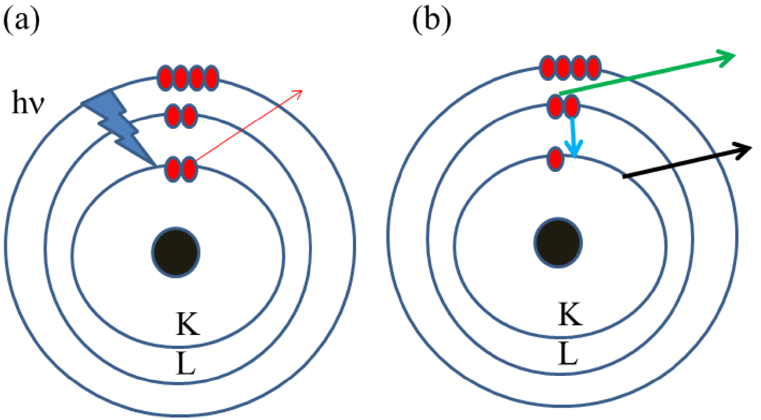
As noticed by the authors, the first three ones, namely AAS, ICP-AES and ICP-MS are quite popular for trace element analysis. In the case of AAS [41], the number of elements detected is quite low even if some recent experimental developments allow the measurements for a significant number of elements. For example, Rello et al. [42] measured Mo and Ti levels in a dried urine spot using solid sampling high resolution continuum source graphite furnace AAS. Unfortunately, the destructive nature of these methods is a strong inconvenience in the case of kidney biopsy. For such biological samples, it is of major importance to localize the calcification: is it present in the glomerulus or in the proximal or distal tubule?
When considering non-destructive techniques, their availability must also be considered. Indeed, regarding PIXE analysis, a source of protons is needed and to date there are only two experimental setups existing in France [43]. Furthermore, the set of non-destructive techniques (Table 2) displays very different sensitivities [40]. Clearly, the limit of detection of SEM–EDS seems to be quite high. Nevertheless, because the dimension of the probe is very small, the presence of trace elements in submicrometer particles can be underlined. The localization of trace elements versus an alteration of the tissue such a tumor can be important to establish a medical diagnosis. One efficient way to be able to decipher the role of trace elements is to detect them with a non-destructive technique which has a great sensitivity and then be able to localize the abnormal deposit accurately in the biological tissue. Such an approach calls for classical XRF spectroscopy and in a second step, to perform such experiments using the synchrotron radiation as a source. In the latter case, the spatial resolution may be optimized at different scales from millimeters through micrometers down to nanometers.
3. Some basic features regarding XRF
XRF relies on the emission of characteristic secondary X-rays emitted from specific atoms after irradiation of the materials by high energy X-ray beam [44, 45, 46, 47]. The first commercial XRF spectrometer was developed in the 1950s [48]. Since then, XRF has attracted increasing consideration in numerous research areas [49].
Methods for trace element analysis
| Technique | Excitation source | Sample preparation | Measurements conditions | Limit of detection (ppm) | Spatial resolution (μm) |
|---|---|---|---|---|---|
| PIXE | Protons | Dehydrated | High vacuum | 1–10 | 1–3 |
| EDS | Electrons | Dehydrated | High vacuum | ≈5000 | ≈0.1 |
| XRF | In lab X-rays | None | Ambient pressure | ≈50 | 30–50 |
| XRF | Synchrotron radiation | None | Ambient pressure | ≈1 | ≈0.01 |
XRF spectrum collected for a biological apatite (bone) linked to a pathological calcification showing the contributions of Ca (Kα = 3.69 keV, Kβ = 4.01 keV), Zn (Kα = 8.64 keV, Kβ = 9.57 keV), Pb (Lα = 10.55 keV, Lβ = 12.61 keV) and Sr (Kα = 14.16 keV, Kβ = 15.84 keV).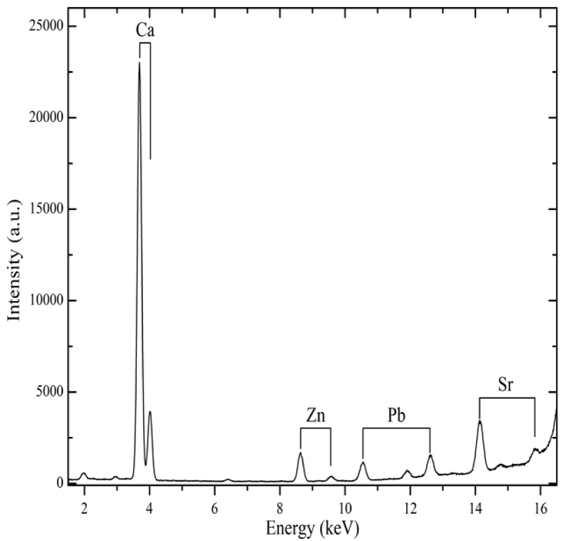
The physical principle of the XRF is illustrated in Figure 1. The excitation of core electrons (present on the K or L shell) of the sample by an X-ray photon leads at the atomic scale to the ejection of an electron called photoelectron (Figure 1a). The formation of a core hole leads to electronic transition which induces the emission of a photon or an Auger electron (Figure 1b). One of the key points of XRF relies on the fact that the energy of the emitted photon is specific to the photo-excited atom [50, 51, 52] (Figure 2, Table 3).
4. Data analysis process procedures
4.1. Experimental facility setup
Nowadays, laboratory XRF setups benefit from up-to-date instrumental developments enabling the detection of trace elements with the highest efficiency (Figure 3). Typical XRF setup includes (i) an X-ray generator with a Cu or Mo anticathode, for example, producing high energy radiation (8.04 keV for Cu anticathode and 17.48 keV for Mo anticathode) allowing the detection of most of the elements of the periodic table, (ii) a multilayer mirror optics focusing a monochromatic beam onto the sample and (iii) a SDD (Silicon Drift Detector) energy dispersive detector (see Figure 3). Further, measurements may also be carried out at a micrometric scale by using microbeams with size down to 20 μm in diameter [53]. The XRF setup, using a sealed tube X-ray source, represents a highly compact instrument which can easily be transported in a hospital.
Characteristic X-ray emission (keV) for selected elements identified in biological samples
| Atomic number | Element | Characteristic X-ray emission line (keV) | |||
|---|---|---|---|---|---|
| Kα1 | Kα2 | Kβ | Lα1 | ||
| 3 | Li | 0.05 | |||
| 6 | C | 0.27 | |||
| 7 | N | 0.39 | |||
| 8 | O | 0.52 | |||
| 9 | F | 0.67 | |||
| 11 | Na | 1.04 | 1.04 | 1.07 | |
| 12 | Mg | 1.25 | 1.25 | 1.30 | |
| 15 | P | 2.013 | 2.01 | 2.14 | |
| 16 | S | 2.30 | 2.30 | 2.46 | |
| 17 | Cl | 2.62 | 2.62 | 2.81 | |
| 18 | Ar | 2.95 | 2.95 | 3.19 | |
| 19 | K | 3.31 | 3.31 | 3.58 | |
| 20 | Ca | 3.69 | 3.68 | 4.01 | |
| 22 | Ti | 4.51 | 5.50 | 4.93 | |
| 24 | Cr | 5.41 | 5.40 | 5.94 | |
| 25 | Mn | 5.90 | 5.89 | 6.49 | |
| 26 | Fe | 6.40 | 6.39 | 7.05 | |
| 29 | Cu | 8.04 | 8.02 | 8.90 | |
| 30 | Zn | 8.63 | 8.61 | 9.57 | |
| 33 | As | 10.54 | 10.50 | 11.72 | |
| 78 | Pt | 9.44 | |||
| 82 | Pb | 10.55 | |||
| 83 | Bi | 10.83 | |||
Laboratory XRF setup at Laboratoire de Physique des Solides (Orsay, France).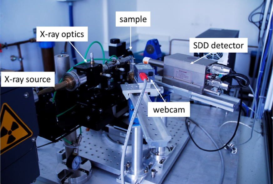
Over the past several years, commercial XRF devices have been developed (see for example the review by Bosco Ref. [54]) and used essentially to detect health problems in people working in the mining and construction industry [55]. Even if their sensitivity is less than thta of the laboratory experimental setup, commercial XRF devices offer the opportunity to gather information “at home” regarding the presence of different heavy elements such as Pb in bone [56], Zn in human toenail clipping [57] and human nail [58], Cr [59] and Fe [60] in skin, Zr in dental restorative resin materials [61], tooth abnormalities (pulp stones) [62, 63, 64], the determination of Fe in blood [65] or the presence of Pu (Plutonium) for workers decommissioning the Fukushima Daiichi nuclear power plant [66].
Practically a portable XRF setup (Figure 4) can be used for solid metals and alloys, ores and soils [67]. Using a gold anode X-Ray generator, under 50 kV high voltage excitation, it offers a powerful source and highly sensitive measurements. Thus the detection limit is lowered for high Z elements and investigation of low Z elements such as Mg, Al, Si and P can be achieved via He purge between the detector and the sample (Figure 4). The spot size is also tuneable from a larger spot of 8 mm diameter to a smaller spot of 3 mm diameter. Furthermore, thanks to a CCD camera, the visualization and location of the areas of interest on the sample is possible. Finally, by connecting the portable XRF with a simple USB cable to a computer, all the data and spectra are fetched from the instrument using a dedicated software for advanced analysis of the results.
Portable X-ray instrument on its portable test stand at the NIMBE-LAPA laboratory (Saclay, France).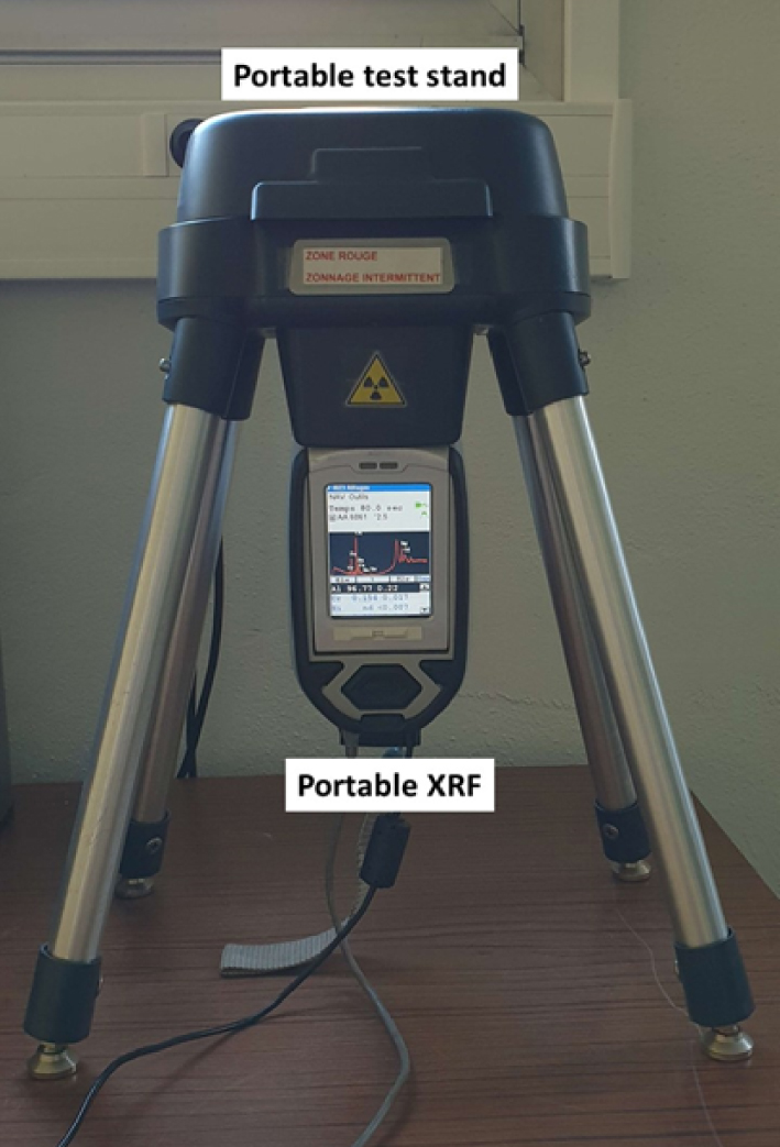
Also noteworthy is the recent development of portable XRF devices that allow assessing the presence of Pu in biological fluids [68, 69, 70]. As underlined by Izumoto et al. [68], fast on-site detection of Pu is usually performed by analysis of α-particles emitted from the adhesive tape peeled off the wound. These authors have developed a new strategy based on XRF where blood is deposited on filter paper. With that experimental procedure using lead as a model for Pu, the XRF signal is proportional to the Pb concentration in blood. With a measurement time of 30 s, these authors estimate the minimum detection limit of Pb in blood collected by filter paper to be 2.4 ppm.
4.2. In vivo investigations based on XRF measurements
At the hospital, in vivo XRF on human tissue can be also considered. Among the early in vivo XRF experiments, the publication of Pavoni et al. [71] discussed the feasibility of in vivo XRF study of the thyroid following stable I (iodine) administration. In vivo XRF analysis of Hg (mercury) in kidney, liver, thyroid, blood and urine has been recently investigated [72, 73]. The mean kidney Hg concentration was 24 μg/g in the exposed workers, and 1 μg/g in the controls. A statistically significant correlation between Hg in the kidney and in urine was found. Also, the Hg levels in liver and thyroid in the exposed workers were below the detection limit.
Experimental setup able to measure the content of Sr in human finger through in vivo XRF measurement.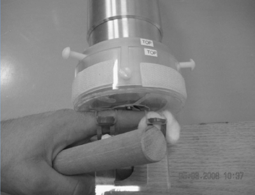
In the case of the work of Moise et al. [74], XRF spectra were collected on the finger and on the ankle bone sites, representing primarily cortical and trabecular bone, respectively (Figure 5). The acquisition time being 30 min, these publications underline the possibility of monitoring and measuring bone Sr (strontium) levels over time.
4.3. XRF using Synchrotron Radiation as a source
The major advantages of using synchrotron sources to do XRF measurements are now discussed [39, 75, 76, 77, 78]. While the brightness of a conventional X-ray tube is around 1010 photons/s⋅mrad2⋅mm2, the corresponding value of synchrotron radiation sources is between 1015 and 1020. The sensitivity of XRF is thus much better when the experiments (Figure 6) are performed on such a large scale instrument [79]. In addition, in the case of synchrotron radiation sources the beam can be focused down to the micrometer or even nanometer scale allowing local analyses [80, 81].
Experimental setup at DiffAbs beamline, SOLEIL synchrotron (St Aubin, France), for (a) standard (300 μm) and (b) microbeam (10 μm) modes. 1: sample holder with translation tables, 2: XRF detector (4 elements SDD), 3:2 dimensions detector for X-ray diffraction (XPAD 3.2) 4: vacuum chamber containing Kirkpatrick–Baez optics, 5: Camera microscope.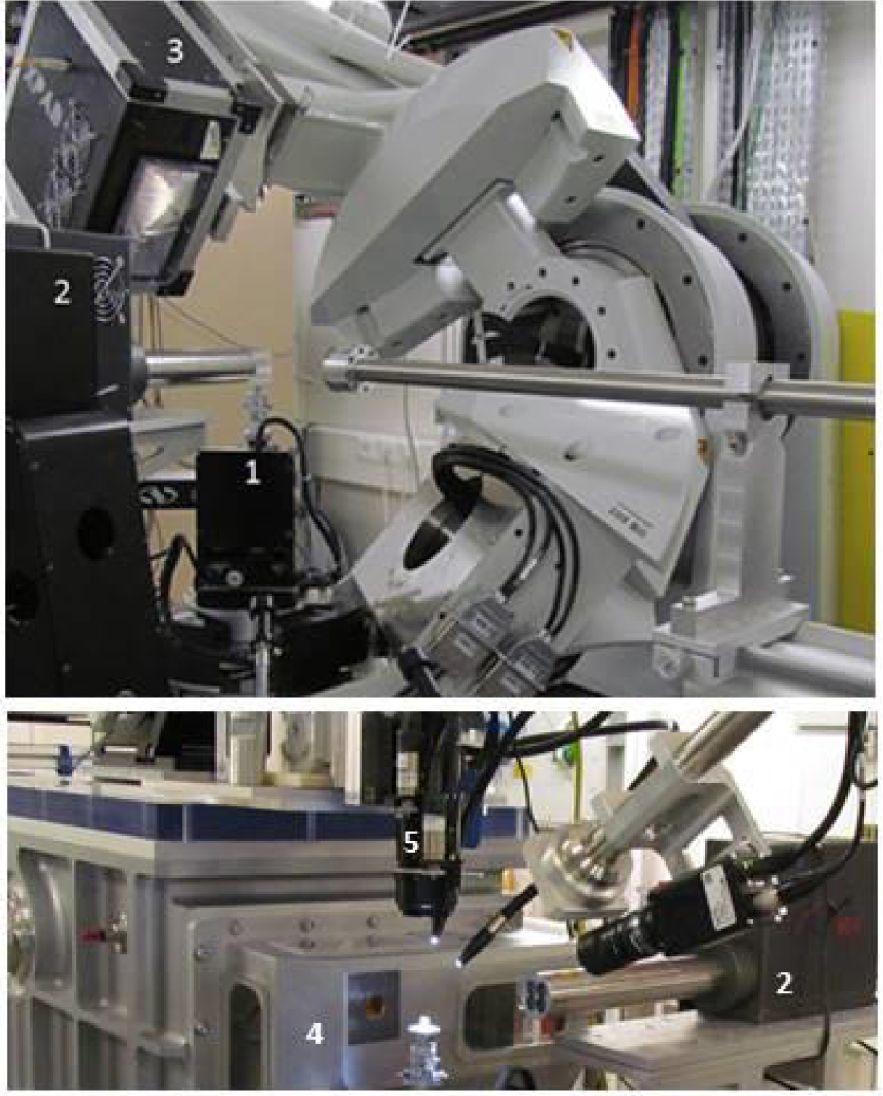
Numerous works have been published on the basis of the subcellular beam size. Among them, a study established the concentration profiles of Fe, Cu, Zn, Br, Sr and Pb in different parts of a tooth in order to discuss the possible influence of diet [82]. It is also possible to acquire 2D maps [83]. In a recent review, Gherase and Fleming [84] present numerous investigations using spatial resolution several micrometers to reveal the distribution of trace elements (<a few μg/g). As underlined by these authors, current research effort is aimed not only at measuring the abnormal elemental distributions associated with various diseases, but also at indicating or discovering possible biological mechanisms that could explain such observations.
Nowadays, there is the possibility to gather information on the spatial distribution of trace elements inside cells [85]. For example, Ortega et al. [86] have developed an original experimental setup which allows aquisition of XRF images with a 90 nm spatial resolution. Such an experimental device leads to important medical results like the accumulation of iron in dopamine neurovesicles. Several major breakthroughs have been achieved using such nanometer spatial resolution [87, 88, 89]. Note that such unique characteristics lead to the conception and the realization of beamline dedicated to medicine (see for example Refs. [90, 91, 92, 93, 94]).
4.4. Data processing and analysis
After the energy calibration of the XRF detector, the very first step of the data processing, which leads to the determination of the spatial distribution of the different elements is given by a fitting procedure of the fluorescence lines for each XRF spectrum. This allows to identify and evaluate the contribution of each element semi-quantitatively. In some cases, the contribution to the measured signal of two elements can be quite close and/or (partially) superimposed and a deconvolution process has to be performed, like in the case of the energy related to Au Lα and Zn Kβ fluorescence emission (Figure 7, from Ref. [95]).
Typical XRF spectrum collected for a biological sample with the contribution of Ca (Kα at 3.691 keV, Kβ at 4.012 keV), Fe (Kα at 6.404 keV, Kβ at 7.058 keV), Zn (Kα at 8.638 keV, Kβ at 9.572 keV). Special attention has been devoted to distinguish, by peak deconvolution, the respective contributions of Zn (Kα = 9.572 keV) and Au (Lα = 9.713 keV) between 9 and 10 keV.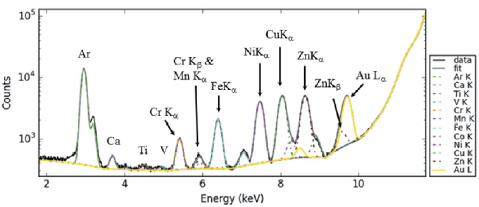
If mapping with XRF contrasts are realized (see e.g., Section 5), visual correlations between the chemical species and their presence in particular regions of the sample can be sometimes noted, but they can also be the result of a subjective view. A more thorough quantitative and statistical analysis is thus expected to support (or not) the visual impression, but also to give more precise information regarding the chemical species identified in the XRF spectra, and to quantify as well the degree of correlation (i.e. any statistical pattern or relationships or even dependence between the datasets). Correlations are useful quantities to be examined, since they can potentially indicate a predictive relationship to be exploited.
Nevertheless, one has to be particularly cautious in drawing conclusions, and several issues have to be carefully considered:
- the smaller the size of the available dataset, the more likely is it to observe a correlation that might not be real and not observable if the same set can be extended. Thus, with small datasets (or small parts of them), correlations can be unreliable.
- presence of single unusual points in the datasets (outlier) can make the computed correlation coefficients highly misleading.
- a correlation between two variables is not a sufficient condition to establish such a causal relationship relating these variables, in either direction.
As previously shown [95, 96, 97, 98], the XRF contrasted maps can be analyzed using Intensity Correlation Analysis methods in order to highlight possible correlations related to the presence of the different chemical elements in a sample. Other correlation coefficients can be used as well, but they will not be discussed here. The reader can also refer to the detailed work of Dunn et al. [98] and references therein.
Let us briefly describe some correlation approaches [99, 100, 101, 102, 103, 104], considering the case of two XRF contrasted images (labeled in the following as image 1 and image 2) of the same lateral size and resolution (same number of points), obtained on the very same sample region, but showing the distribution of two different chemical elements. Xi,j and Yi,j are the intensity of the pixel of coordinates (i,j) for the two images, respectively.
- In a first step, scatter plots can be used. If one expects that the dataset of image 2 (Yi,j) is somehow dependent of the one in image 1 (Xi,j), plotting them as a scatter plot (using Y and X axis respectively) allows drawing some conclusions: (i) a positive correlation between X and Y variables is found if the obtained pattern exhibits a positive slope (from lower left to upper right of the graph, i.e. the Y variable tends to increase when the X variable is increasing); (ii) a negative correlation is found if the above mentioned trend is opposite; (iii) no correlation generally translates into no trends noticed in the scattered plots. Possibly, the result can be fitted (but no “universal” model exists) and the degree of correlation can thus be quantified by the parameters of the fit and their comparison between similar datasets.
- The Pearson colocalization coefficient for two variables is defined as the ratio of the covariance of the two variables by the product of their standard deviation:
with the summations being performed over the entire considered dataset/image, i.e., all the pixels of coordinates , and Xave and Yave denoting the average intensity for the two images, respectively.The interpretation of the results based only on the Pearson coefficient might give rise to controversy: the results are rather sensitive to noise and are reliable only for high correlation (which is not always the case in experiments).
- In order to push this analysis further, other coefficients and correlation maps can be calculated. Pearson correlation coefficient is a symmetric quantity, which can be a limitation in the interpretation of the results. To overcome this issue, the Manders’ (colocalization) coefficients M12 and M21 allow to know, for M12, how well the intense pixels in image 1, which are above a certain intensity threshold, colocalizes with intense pixels in image 2 (i.e. the probability to find bright pixels, above a certain threshold value, in image 2 only at the positions of intense pixels in image 1) and vice versa for M21. When using this approach, a threshold for the XRF signal needs to be used to calculate M12 and M21 [84]; for each image, it was set to half of the average signal, average calculated over the whole image.
Denoting the threshold values of X and Y images by 𝜏x and 𝜏y respectively (their values can be 0 as well), this can be written as:
The last two approaches mentioned above (Pearson and Manders coefficients) are not equivalent, and give complementary information. Also, note that the Manders coefficients are not necessarily symmetric. For example, it might be that a great part (or all) of the intense pixels of image 1 corresponds to intense pixels in image 2 (M12 ∼ 1), but the opposite might not be true: regions of the bright signal in the second image might not have any correspondence to image 1 (M21 ≪ 1). An example is shown in Section 6.6.
All the correlation/colocalization approaches might have advantages and drawbacks—none of them should a priori be considered better than the other. A careful examination is always needed and the choice of one approach over the other largely depends on the particular sample, datasets available and the question(s) to be addressed. A tentative workflow to guide the researcher in identifying and applying the proper (or better) technique can be found in [98].
5. Sample preparation
The characterization of trace elements present in biological samples is not easy. Some problems may come from washing process which may change significantly the location of diffusible trace elements. Forty years ago, Stika et al. [105] underlined the necessity of low temperature preparative procedures for diffusible ion localization using the ion microscope. Using conventional fixation procedures, these authors have observed significant ion loss and redistribution which exceeded the 1 μm lateral resolution. More recently, Porcaro et al. [106] distinguished two major bias that can be encountered under X-rays. First is the modification of the native chemical species during sample processing, and second the alteration of chemical species during XAS analysis, due to beam irradiation damage. Following the publication of Bacquart et al. [107] the use of cryogenic conditions for sampling followed by the storage in an inert atmosphere all along the analytical process is highly advocated to preserve the initial chemical species. Keeping the sample at low temperature also during the analysis offers the supplementary advantage to limit the irradiation damage and to reduce the element loss that is induced by intense beam irradiation, especially when a focused beam is used. For our experiments, biological tissue were embedded in paraffin, three to five microns slices were deposited on low-e microscope slides (MirrIR, Kevley Technologies, Tienta Sciences, Indianapolis). The paraffin was then chemically removed (xylene 100% for 30 min to 4 h) in order to improve the crystal detection under the microscope. Note that as underlined by Pushie et al. [4], the possibility for altered chemical speciation, elemental redistribution, leaching, or contamination from the long list of reagents or preparation steps used in paraffin and methacrylate embedding processes should always be considered.
6. Scientific cases
6.1. Biomarker in biological fluids
Several kinds of biological fluids namely blood [108, 109, 110], amniotic fluid [111], urine [112], semen [113], saliva [114], sweat [115] can be investigated by XRF. As noticed by Langstraat et al. [116], human blood can be analyzed using XRF through the presence of elements K, Cl and Fe. In the case of semen, the significant elements are K, Cl and Zn. For saliva, the element K can be underlined, and finally urine and sweat contain K, Cl and Ca [117].
For the clinician, a major question is related to the selection of the best non-invasive biomarker to perform XRF experiments. To identify the best human biomarkers for Sb exposure, Ye et al. [118] have analyzed 480 environmental samples from an active Sb mining area in Hunan, China. For this study, they consider urine, saliva, hair and nails, the drinking water being the more important contribution (85–100% of the average daily dose—ADD). The authors found a positive correlation between ADD and Sb content in hair (p = 0.02), but not in urine (p = 0.051), saliva (p = 0.52) or nails (p = 0.85), suggesting that hair is the best non-invasive biomarker.
Finally, XRF may bring valuable information to the sports medicine physician. In a recent study, Jablan et al. [119] explored the impact of endurance exercise on urinary level of trace elements such as Ca, P, K, Na, Se, Zn, Mn, Cu, Fe and Co using the bench top Total Reflection XRF (TXRF) spectrometer. The results underline that the level of Co increased ten-fold after the race. Such observation/conclusion is in line with the fact that Co helps assimilation of Fe and hemoglobin synthesis inducing erythropoiesis, and consequently enhances endurance [120].
6.2. Highlighting heavy elements in drugs
It is known that several drugs contain heavy elements in their chemical composition [121, 122], as Pt, Cu and Sr cited in the following examples. As underlined by Johnstone et al. [123], since the discovery of cisplatin by Rosenberg in 1960 [124], Pt-based drugs became a mainstay of cancer therapy. More precisely, approximately half of all patients undergoing chemotherapeutic treatment receive a Pt drug namely cisplatin (cis-[Pt(II) (NH3)2Cl2]), carboplatin and oxaliplatin [125]. Recently, some authors demonstrated that inhibition of dengue virus serotype 2 in Vero cells can be obtained with [Cu(2,4,5-triphenyl-1H-imidazole) 2(H˙2O)2] ⋅ Cl2 [126]. Sr-based drugs increase bone mass in postmenopausal osteoporosis patients and reduce fracture risk [127, 128, 129, 130, 131].
(a, b) Zn and Pt XRF maps collected in the case of a human kidney biopsy (from Ref. [97]); (c, d) Zn and Pt XRF maps collected in the case of female mice (from Ref. [132]). Scanned area 16 × 16 μm, beam dimensions 50 × 50 nm2, 50 nm step size, measurement time 0.1 s per point, primary beam energy 17.5 keV; (e–g) (from Ref. [133]) cell morphologies obtained by Nomarski are shown at x100 magnification, each field of view is equivalent to an area of 70 × 70 μm, Zn and Pt maps obtained using SXFM.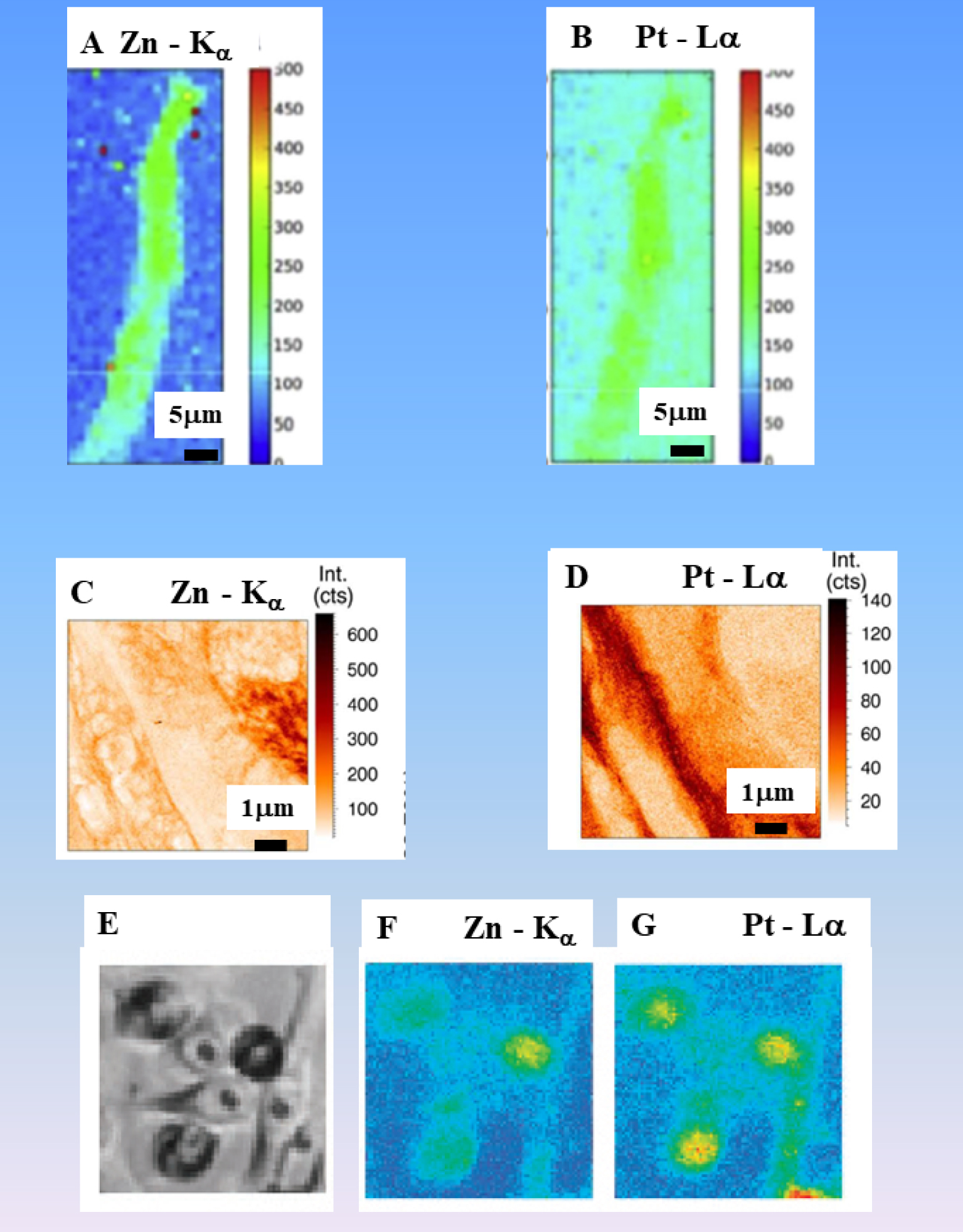
Disorders due to an accumulation of Mn, Cu, or Fe and causing neurotoxicity, OMIM is for Online Mendelian Inheritance in Man
| Disorders | Transition metal | Inheritance | Gene | OMIM | Gene function | Symptoms |
|---|---|---|---|---|---|---|
| Hypermanganesemia with dystonia 1 | Mn | Autosomal recessive | SLC30A10 | 613280 | Manganese transporter | Dystonia, cock-walk gait Parkinsonism |
| Wilson’s disease | Cu | Autosomal recessive | ATP7B | 277900 | Copper transporter | Dysarthria, dysphagia, tremor, dystonic rigidity |
| Acaeruloplasminaemia, Cerebellar ataxia, Hypoceruloplasminemia | Fe | Autosomal recessive | CP | 604290 | Ferroxidase | Chorea, ataxia, dystonia, Parkinsonism, Diabetes mellitus |
In a recent study, Esteve et al. [96, 97] have shown that it is possible to detect Zn and Pt in kidney biopsy of patients (Figures 8a, b). In one case, the detection of Pt was made six days after the last oxaliplatin injection, while for the second case, the biopsy was performed more than 15 days after the first drug injection and several dialysis. Using nano-XRF spectroscopy, Laforce et al. [132] examined the Pt distribution in ovarian tissues. The measurements proved that Pt resides predominantly outsides the cancer cells in the stroma of the tissue (Figures 8c, d). Figures 8e–g, report some images from the paper of Shimura et al. [133]. Scanning XRF microscopy (SXFM) allows to map intracellular elements after treatment with cis-diamminedichloroplatinum(II) (CDDP), a Pt-based anticancer agent. A precise analysis of several spatial repartitions regarding Pt and Zn, reveals that the average Pt content of CDDP-resistant cells was 2.6 times less than that of sensitive cells, and the Zn content was inversely correlated with the intracellular Pt content.
This approach can be extended to drugs without heavy elements but with advanced materials, namely mesoporous silica [134] or gold nanostructures [135], that are able to enhance treatment. In such design for the drug, XRF also gives the possibility to localize the drug through gold quantum dots precisely inside the organ [95] or in a cell [136]. Finally, it is clear that such an approach can help the clinician to establish a heavy metal intoxication diagnosis and to understand more deeply the toxicity mechanism [137].
6.3. Diseases related to a metal dysregulation
As underlined by Umair and Alfadhel [138], genetic disorders associated with metal metabolism constitute a vast group of disorders [139], mostly resulting from defects in the proteins/enzymes involved in nutrient metabolism and energy production. Table 4 gives some physiological details regarding several genetic disorders [139]. Such genetic disorders may lead to accumulation of heavy elements. For example, the accumulation of Fe [140], Mn [141], Cu [142], Se [143] or Zn [144] in brain induces severe neurodegeneration. XRF was used to investigate several diseases related to a metal dysregulation. Among them Menkes disease [145, 146] is linked to a Cu deficiency and Wilson disease [147] is related to an accumulation of Cu in tissues.
In the first case and to estimate the standard therapy, Kinebuchi et al. [148] have evaluated the Cu distribution at subcellular level of resolution in the treated classic Menkes disease patients through XRF. A careful analysis of the data indicates that a standard therapy supplies almost enough Cu for patient tissues but passes through the tissues to venous and lymph systems. Regarding Wilson’s disease, different studies were performed through XRF [34, 149] or through LA-ICP-MS [150] to determine the Cu concentration in tissues. A recent study clearly showed that XRF is more sensitive than staining procedure used routinely at the hospital [34]: a laboratory-based XRF spectrometer is sufficient to reveal the excess of Cu in tissues.
Typical XRF spectrum collected for a kidney stone showing clearly the contributions of Al (Kα ≈ Kβ = 1.487 keV). Contributions coming from other elements such P (Kα = 2.01 keV, Kβ = 2.14 keV) or Cl (Kα = 2.62 keV, Kβ = 2.81 keV) can be also identified.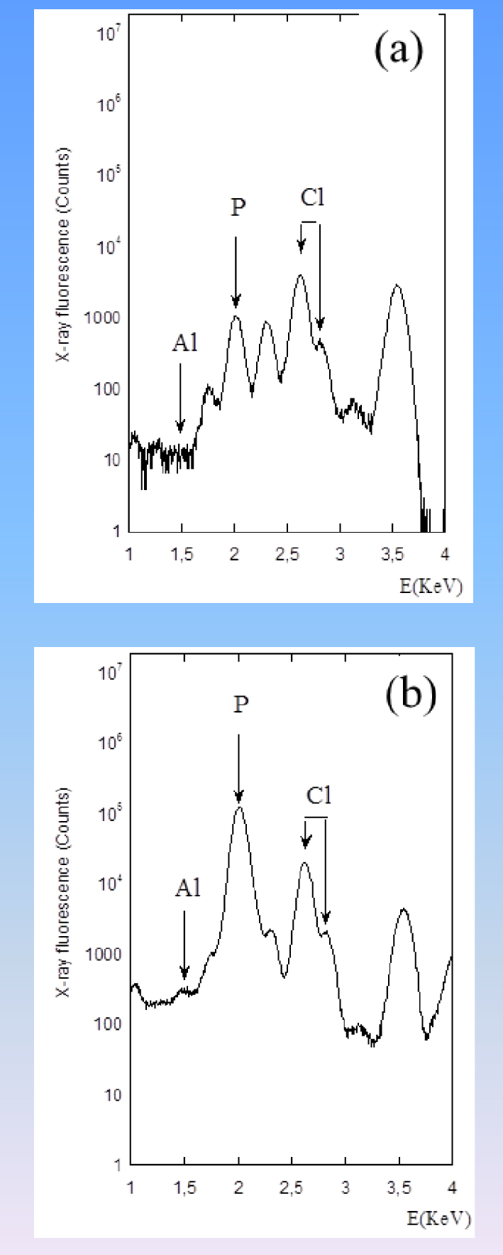
6.4. Diseases related to the adsorption of toxic elements
Recently, different investigations have underlined a high content of nephrotoxic elements such as Al [151, 152, 153] and Mn [154] in green tea leaves. While daily intakes of Al present in food were estimated as 2 ± 6 ng for children and 9 ± 14 ng for adults [154], several studies reported that in some of the tea infusions, toxic metals exceed the maximum permissible limits stipulated by different countries [155]. For example, levels of Al stipulated were 0.06–16.82 mg⋅L−1. Moreover, among the different human diseases related to Al [156], it seems that Alzheimer’s disease is associated with the presence of Al [157, 158] and thus the high Al content in tea is a matter of concern.
XRF measurements performed on kidney stones reveal some Al contribution (Figure 9). Works are in progress to establish a correlation with the consumption of tea [159, 160]. Note that tea leaves contain calcium oxalate and that calcium oxalate (monohydrate and dehydrate) have been identified in kidney stones [161].
Correctly positioned double J stent. References: Clinical center ”Dr Dragisa Misovic-Dedinje”—Belgrade/RS.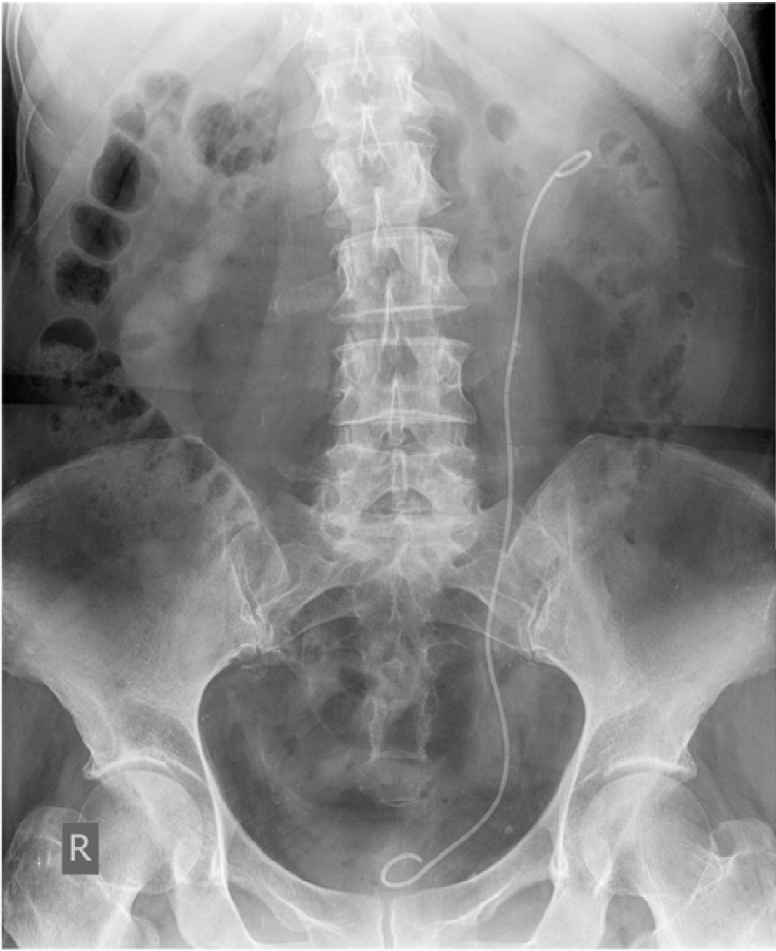
6.5. Heavy elements in medical devices
Medical devices may contain heavy elements and their possible release constitutes a real health problem [162]. Orthopedic implants [163, 164], JJ stents [165, 166, 167] or dental implants [168, 169] contain heavy elements. Regarding orthopedic implants, several investigations have underlined the presence of oxide particles containing Cr [170, 171, 172] in tissues around retrieved metal on metal implants. Considering JJ stents are made of polymeric biomaterials, in order to verify the location of this medical device in the urinary system through X-ray radiography (Figure 10), heavy elements namely Ba [173], Bi, Ta or W may be added [174]. The release of such elements may lead to pathologies and it is thus crucial to determine their nature, which can easily be done by XRF measurements (Figure 11).
Presence of Bi and S in a JJ stent underlined by XRF.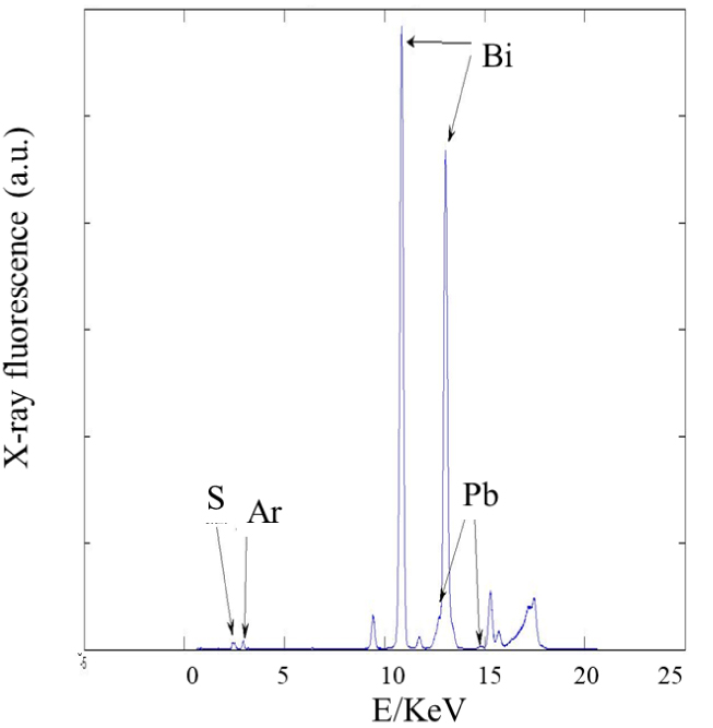
In order to investigate the possible release of Fe and Cr from orthopedic implants, Ektessabi et al. [175] have performed XRF experiments. The complete set of data showed that some elements of the implant namely Ti, Fe and Cr are present in the prosthesis. Similar results regarding the contamination by metallic elements released from joint prostheses were obtained by PIXE [176].
6.6. The case of tattoos
Tattooing has gained tremendous popularity in Western countries where approximately 10% of the populations have at least one tattoo. In fact, the tattoo prevalence overseas and in Europe is even higher, especially among the youth, for whom it is up to 15–25% according to the country [177]. The presence of different metals including Ti, Fe, Cr or Zn have been identified in the chemical composition of tattoo’s ink [178]. Those elements, injected into the dermis, remain lifelong in the skin [179]. Moreover, recent data show that these inks contain metals incorporated in nano- and submicron particles [180]. Such chemical and structural characteristics of the inks used for tattoos may explain why, as reported by Kluger [181], many complications are related to tattoos encompassing ink allergy, benign or malignant tumors. It is thus of primary importance to determine the chemical nature of organic and inorganic elements within tattoo inks and the spatial distributions of these elements within the skin reactions to tattoos. XRF experiments were performed to attain these goals, such spectroscopy being able to determine and localize the heavy elements versus some specific structures of the tissue [182, 183, 184, 185, 186].
In a recent study, a set of tattooed patients suffering from skin cancer was considered [187]. Indeed, several types of carcinogenic compounds were identified in tattoo inks, including primary aromatic amines (PAA), cleavage products of organic azo-colorants. An analysis of the medical literature indicates a possible association between skin cancers including cases of keratoacanthoma (KA) and the use of red inks [188].
The clinical and histopathological data from three patients diagnosed with tattoo associated KA indicate that they have developed KA on red ink within several weeks following the tattoo setup procedure. Histopathological data indicate the presence of intra-dermal red pigments, located in the direct periphery of the tumoral mass. XRF maps acquired on the different biopsies revealed elemental distribution and it was able to discuss more deeply the relationship between KA and the chemical composition/distribution of tattoo ink. Observation through an optical microscope (Figure 12a), shows mainly pink and black inks in the superficial and deep dermis.
(a) HES (Hematoxylin Erythrosine Saffron)-stained image obtained using ×25 magnification. Raster maps with XRF contrast corresponding to (b) Ca (intensity with a maximum equal to 20), (c) Ti (intensity with a maximum equal to 1000), (d) Fe (intensity with a maximum equal to 60), (e) Cu (intensity with a maximum equal to 200) and (f) Zn (intensity with a maximum equal to 140) respectively. Three regions of interest (ROIs) are also highlighted, and will be used in the following for the analysis. The color scale is linear (from blue to red), and spans from 0 to the above reported maximum value for each map.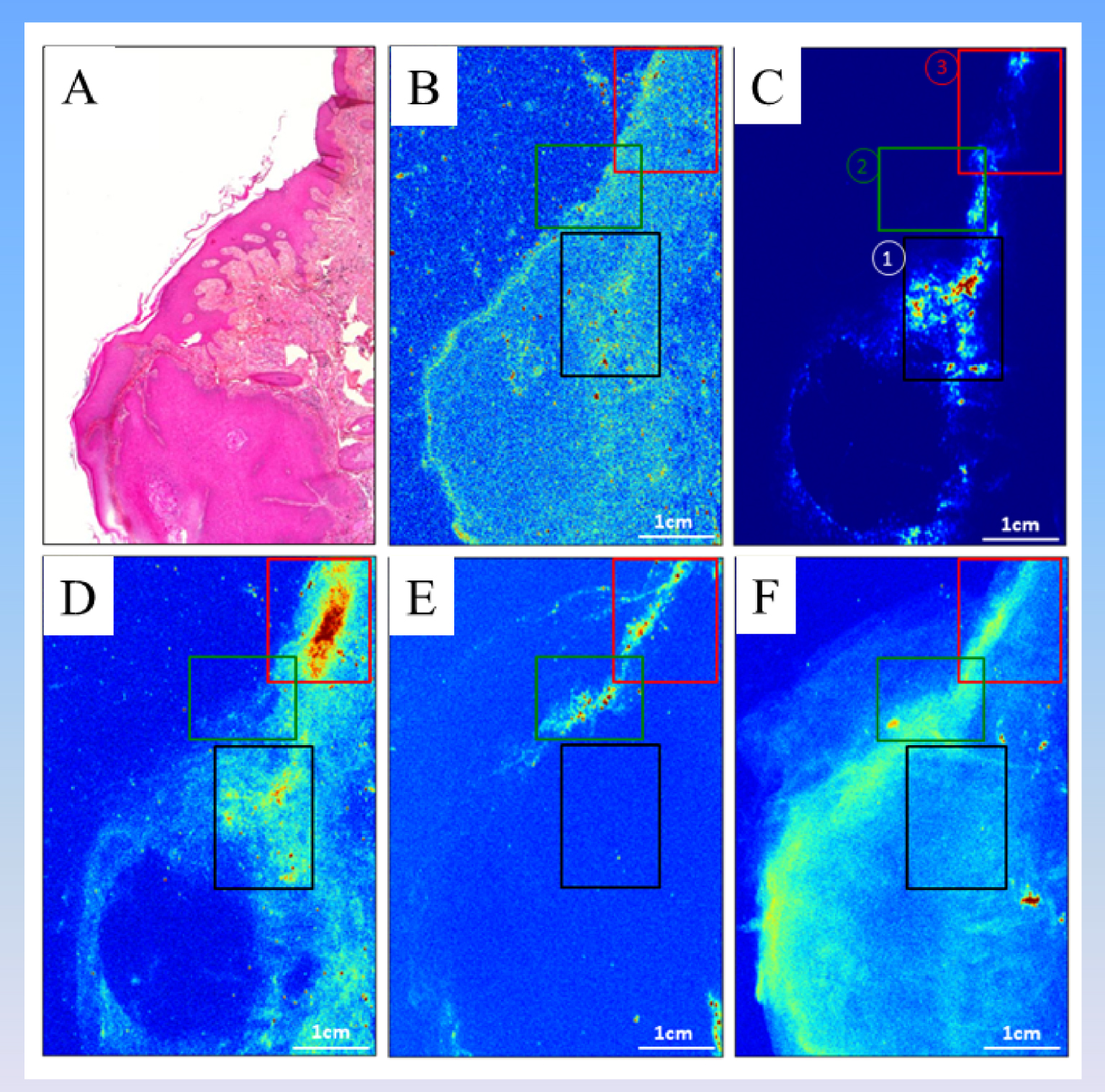
In order to illustrate the quantitative results that can be obtained from the XRF contrast maps obtained on the biopsies and collected on the DiffAbs beamline (SOLEIL Synchrotron), they are analyzed using the above detailed approaches (see Section 4.4). The analysis can be, of course, performed on the full dataset (XY map) or regions of it. Figure 12 (b to e) shows XY raster maps with XRF contrast corresponding to various elements.
The correlation analysis was performed for all the possible resulting combinations of the situations mentioned above (more than four elements, for full image and three ROIs), but we will give in the following as a detailed example, two situations: correlations of XRF maps with Ti–Fe and Ti–Zn contrasts only for ROI no. 1 (cf. Figure 12). The results are shown in Figure 13 (a and b panels respectively).
Analysis performed for ROI no. 1/XRF maps with (a) Ti–Fe and (b) Ti–Zn contrasts. The scatter plots are shown, with the dotted lines being guides for the eye; the insets show the respective zooms on the used ROIs of the XRF maps. The calculated Pearson (P) and Manders (M) coefficients are (a) P(Ti–Fe) = 0.51, M(Ti–Fe) = 0.89, M(Fe-Ti) = 0.59 and (b) P(Ti–Zn) = −0.11, M(Ti–Zn) = 0.98, M(Zn–Ti) = 0.53 (see also Tables 5 and 6).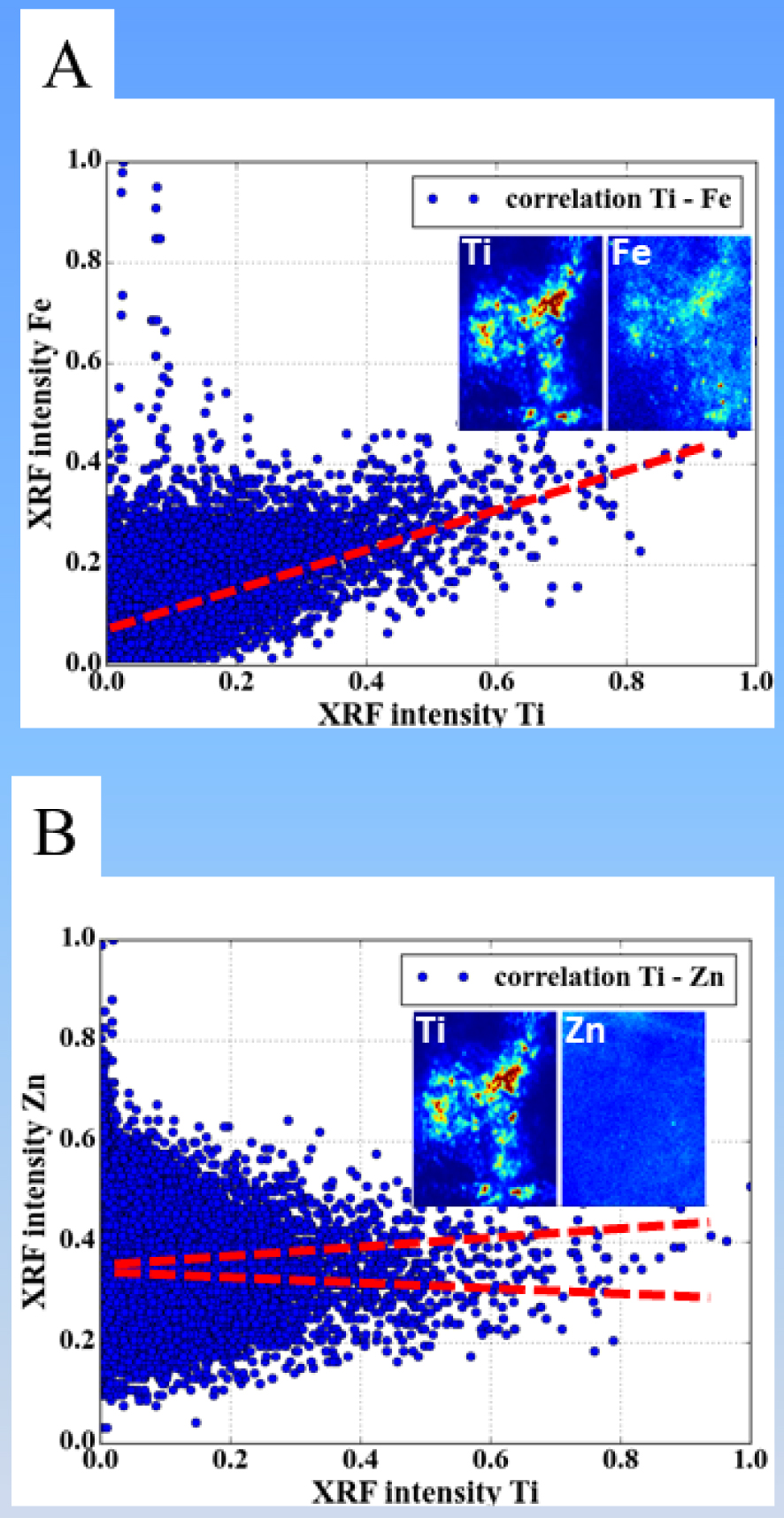
For the Ti–Fe XRF maps (Figure 13a), the scatter plot shows a positive correlation, which is confirmed by a positive Pearson coefficient. Visual examination of the XRF maps also show that the same areas of the ROI seem to exhibit both Ti and Fe signal. Nevertheless, it is the use of the Manders coefficients which allow quantifying the co-existence of the Ti and Fe in this region: with a value of M12 = M(Ti–Fe) = 0.89, the probability to find Fe at each point where Ti is present is rather large (almost 90%). The inverse situation is slightly less favorable: the probability to find Ti at each point where Fe is present is slightly smaller, amounting to only ∼60%. Such a result is difficult to argue by simple visual examination of the data, if no mathematical quantification is performed.
It is a little bit more complex to interpret the Ti–Zn XRF maps (Figure 13b), if one uses only scatter plot and Pearson coefficient. The scatter plot does not really allow to conclude a positive or negative correlation, while the slightly negative Pearson coefficient (−0.11) would suggest that the presence of the two chemical species is slightly anti-correlated in the considered ROI. A careful examination of the XRF maps and noting that the Zn signal seems to be approximately uniformly distributed in the considered ROI is confirmed by the calculated Manders coefficients: M(Ti–Zn) amounts almost unity, showing that in any sample point (in ROI no.1) where Ti is present, Zn is also detected. The reverse is not anymore true; M(Zn–Ti) is of about 50%. Considering that Zn is present over the whole ROI no.1 area, this corresponds to a presence of the Ti in only approximately half of this region of the sample.
Tables 5 and 6 below show the obtained results (Pearson and Manders coefficients) for the different chemical element combinations and different considered ROIs. The first chemical element (el.1) is reported on the first (leftmost) column, and the second one (el.2) on the first (topmost) row.
Calculated Pearson coefficients for different pairs of chemical elements (el.1, el.2)
| el.1\el.2 | Ca | Ti | Fe | Cu | Zn |
|---|---|---|---|---|---|
| Ca | ⊠ = 0.07 | ⊠ = 0.04 | ⊠ = 0.07 | ⊠ = 0.05 | |
| xxx | ① = 0.11 | ① = 0.05 | ① = 0.03 | ① = 0.02 | |
| xxx | ② = 0.03 | ② = 0.11 | ② = 0.07 | ② = 0.23 | |
| ③ = 0.01 | ③ = 0.07 | ③ = 0.05 | ③ = 0.05 | ||
| Ti | ⊠ = 0.16 | ⊠ = −0.00 | ⊠ = 0.01 | ||
| xxx | xxx | ① = 0.51 | ① = 0.04 | ① = −0.11 | |
| xxx | xxx | ② = 0.47 | ② = −0.11 | ② = −0.16 | |
| ③ = 0.10 | ③ = 0.16 | ③ = 0.13 | |||
| Fe | ⊠ = 0.07 | ⊠ = 0.03 | |||
| xxx | xxx | xxx | ① = −0.01 | ① = −0.01 | |
| xxx | xxx | xxx | ② = 0.05 | ② = 0.16 | |
| ③ = −0.09 | ③ = 0.05 | ||||
| Cu | ⊠ = 0.08 | ||||
| xxx | xxx | xxx | xxx | ① = 0.04 | |
| xxx | xxx | xxx | xxx | ② = 0.30 | |
| ③ = 0.35 | |||||
| Zn | xxx | xxx | xxx | xxx | xxx |
| xxx | xxx | xxx | xxx | xxx | |
⊠ = Full image, ① = ROI1, ② = ROI2, ③ = ROI3. The values of the coefficients are colored according to the following color map: black [ <0.0]; blue [0.0–0.1]; green [0.1–0.2]; orange [0.2–0.3]; red [ >0.3].
Calculated Manders coefficients for different pairs of chemical elements (el.1, el.2)
| el.1\el.2 | Ca | Ti | Fe | Cu | Zn |
|---|---|---|---|---|---|
| Ca | ⊠ = 0.227 | ⊠ = 0.566 | ⊠ = 0.221 | ⊠ = 0.815 | |
| xxx | ① = 0.563 | ① = 0.817 | ① = 0.181 | ① = 0.985 | |
| xxx | ② = 0.163 | ② = 0.600 | ② = 0.351 | ② = 0.868 | |
| ③ = 0.321 | ③ = 0.691 | ③ = 0.335 | ③ = 0.848 | ||
| Ti | ⊠ = 0.701 | ⊠ = 0.786 | ⊠ = 0.167 | ⊠ = 0.978 | |
| ① = 0.595 | xxx | ① = 0.889 | ① = 0.184 | ① = 0.983 | |
| ② = 0.695 | xxx | ② = 0.982 | ② = 0.209 | ② = 0.898 | |
| ③ = 0.705 | ③ = 0.940 | ③ = 0.331 | ③ = 0.965 | ||
| Fe | ⊠ = 0.622 | ⊠ = 0.306 | ⊠ = 0.213 | ⊠ = 0.887 | |
| ① = 0.562 | ① = 0.593 | xxx | ① = 0.179 | ① = 0.986 | |
| ② = 0.632 | ② = 0.243 | xxx | ② = 0.376 | ② = 0.918 | |
| ③ = 0.667 | ③ = 0.414 | ③ = 0.250 | ③ = 0.925 | ||
| Cu | ⊠ = 0.492 | ⊠ = 0.165 | ⊠ = 0.431 | ⊠ = 0.684 | |
| ① = 0.541 | ① = 0.541 | ① = 0.776 | xxx | ① = 0.986 | |
| ② = 0.548 | ② = 0.095 | ② = 0.557 | xxx | ② = 0.942 | |
| ③ = 0.584 | ③ = 0.351 | ③ = 0.634 | ③ = 0.842 | ||
| Zn | ⊠ = 0.577 | ⊠ = 0.233 | ⊠ = 0.557 | ⊠ = 0.212 | |
| ① = 0.545 | ① = 0.530 | ① = 0.793 | ① = 0.183 | xxx | |
| ② = 0.526 | ② = 0.135 | ② = 0.528 | ② = 0.392 | xxx | |
| ③ = 0.675 | ③ = 0.350 | ③ = 0.763 | ③ = 0.303 | ||
⊠ = Full image, ① = ROI1, ② = ROI2, ③ = ROI3. The values of the coefficients are colored according to the following color map: black [0.0–0.2]; blue [0.2–0.4]; green [0.4–0.6]; orange [0.6–0.8]; red [0.8–1.0].
The values of the Manders coefficients M(X–Zn) (X = Ca, Ti, Fe, Cu) are typically larger than 80% (with exception in the case of X = Cu/full image, but still with a significantly large value of 68%). This result implies that whatever the chemical element X is, when detected on the XRF maps or ROIs, the Zn is systematically present as well. This is somehow expected and in full agreement with the observed rather uniform distribution of Zn over major part of the XRF map (or at least the regions where the other elements are present), as it can be visually detected in Figures 12 and 13. It is only in the case of X = Cu (and full image) that probably there are some areas of the sample where the presence of the Cu is not correlated with the one of the Zn.
Another interesting case to be discussed is the correlation of Ti and Fe. The large values (about 80 to 90%) for Manders coefficient M(Ti–Fe) indicates that the presence of Ti is systematically accompanied by the presence of Fe. The reverse is not true, and, depending on the chosen area to be investigated, in regions with detected Fe, the Ti can also be detected/correlated with probabilities ranging from 25 to 60%.
Another case which might be worthwhile to be noticed: Cu–Fe, with M(Cu–Fe) ∼60% and M(Fe–Cu) ∼30%. It shows that in areas with detected Cu, the probability to find Fe is rather high (60%), but the reverse (finding Cu in Fe rich areas) is much less probable (30%).
From a medical point of view, these spatial correlations between heavy elements can be related to at least three different aspects. The first one is related to the mixing of pigments which is made to obtain the color of the tattoos. For example, orange or light red is a mix between red (iron oxide) and white (TiO2 or ZnO) [180]. A second aspect is linked to the fact that a heavy element can trigger inflammation process in the skin, leading to the co-location of exogenous heavy metal (TiO2 for example) present in the ink and Zn, an element of metalloproteins which are engaged in cutaneous inflammation [189]. Finally, inflamed tissues are usually associated to increased blood vascularization. There is hence a possibility to have a superposition of exogenous heavy metals and the accumulation of blood which contains iron. To explore those three aspects, we have to know if iron and zinc have an endogenous or an exogenous origin. Such information is not available by XRF but could be by X-ray absorption spectroscopy [190, 191, 192].
In the case of Ti, its exogenous origin is obvious. TiO2 was associated with a low toxicity particle but this view changed after The International Agency for Research on Cancer (IARC) indicated that TiO2 is possibly carcinogenic to humans [193]. Here, XRF data have detected a significant presence of TiO2 around the tumor, and underlining a possible cancerogen effect of this metal [187].
Zhang et al. [194] have compared regular TiO2 particles (including fine nano-TiO2 and microsize nano-TiO2) and nano-TiO2 particles and showed that nano-TiO2 particles have a stronger catalytic activity. Quite recently, Xue et al. [195] explored the cytotoxicity and oxidative stress induced by nano-TiO2 under UVA irradiation with different crystal forms (anatase, rutile and anatase/rutile) and sizes (4 to 60 nm) in human keratinocyte HaCaT cells. Their results indicated that anatase and amorphous forms of nano-TiO2 showed higher cytotoxicity than the rutile form. More precisely, nano-TiO2 could induce the generation of reactive oxygen species ROS and damage HaCaT cells under UVA irradiation. Under irradiation, it is well known that TiO2 may generate a significant quantity of ROS which play important roles in the modulation of cell survival, cell death, differentiation, cell signaling, and inflammation-related factor production [196]. Finally, Ross et al. [197] have underlined another aspect regarding the relationship between TiO2 and tattoo showing that TiO2 is overrepresented in tattoos that respond poorly to laser treatment.
7. Synergy with other physicochemical techniques
While XRF and other techniques (see part 2: AAS, ICP-AES, ICP-MS…) reveal the nature and concentration of the heavy elements present in biological samples, it can be interesting to the clinician to know in which chemical phases these heavy elements reside.
To attain this goal, different complementary techniques can be selected. The first ones are classic in-lab techniques. Among them, Raman plays a key role. For example, in the case where Ti is revealed in skin tattoos, it allows to distinguish between two Ti oxide polymorphs namely rutile and anatase [198, 199]. The Raman spectra clearly pointed out the presence of the rutile polymorph for a patient who presented a keratoacanthoma (Skin cancer) [187]. Such complementary information can be obtained with Raman spectroscopy for other elements such Zn [200] or Fe [201]. It is worthwhile to underline that in the case of Fe, Mossbauer spectroscopy constitutes a powerful technique to discriminate between all the different Fe oxides [202, 203] and that spectroscopy may be associated with a spatial resolution of ∼10–20 μm [204].
Complementary structural information is available through X-ray Absorption Near Edge Structure (XANES) spectroscopy to determine the structure around elements previously detected by XRF [190, 191, 205]. When Cr is detected, it is of primary importance to know the oxidation state of this element. While Cr(III) serves as a nutritional supplement, and may play a role in glucose and lipid metabolism, Cr(VI) is very toxic inducing a wide variety of injuries in cells, such as DNA damage [206]. Through XANES spectroscopy, Ortega et al. [207] have shown that soluble Cr(VI) compounds are fully reduced to Cr(III) in cells. XANES spectroscopy can bring complementary valuable information also in the case of nanometer scale metallic particles [208, 209, 210, 211], a nanomaterial which have numerous applications in medicine [212, 213, 214].
X-ray diffraction (XRD) can also be used to reveal the long range structure of compounds [215, 216, 217, 218, 219, 220, 221]. Among the different investigations which are based on the association between XRD and XRF spectroscopy [222, 223, 224, 225, 226], we can quote the determination of the chemical composition of microcalcification, present in cartilage, which was obtained using XRD on selected points corresponding to high concentration of Ca as defined by XRF spectroscopy [227].
8. Conclusion
The scientific cases presented above, regarding the opportunities of XRF in medicine, show clearly that XRF now plays a key role in establishing a diagnosis or in understanding deeply the interaction between heavy elements and human tissues at the subcellular level. Even if the sensitivity of such a technique is higher when synchrotron radiation is used as a source [228], this technique can be used in hospitals, using portable instrument or laboratory setup, giving almost in real time the nature and the concentration of the different elements present, even at trace levels.
Acknowledgments
This work was supported by the Physics and Chemistry Institutes of CNRS and by contracts ANR-09-BLAN-0120-02, ANR-12-BS08-0022, ANR13JSV10010-01, convergence UPMC CVG1205, Labex Matisse, Labex Michem and CORDDIM-2013-COD130042. The authors are grateful to the SOLEIL Synchrotron Facility and ESRF for beam time allocation and would like to very much thank the support groups and beamline teams of SOLEIL and ESRF for their help during experiments.