

1 Introduction
In karst hydrology, the transport of particles is a complex process involving the phenomena of direct transfer, deposition, and resuspension [3,8,19,22,23,29,30]. At the flood scale, the turbidity observed has two possible origins: (i) an allochthonous origin, corresponding to the direct transfer of particles from the inlet to the outlet of the karst system, and (ii) a autochthonous origin, associated with the resuspension of intrakarstic sediment previously deposited within the karst network.
Turbidity, water discharge, and electrical conductivity (T, D and EC) data have been used extensively to investigate transport properties (direct transfer of ground or surface water, deposition of suspended particulate matter, resuspension of intrakarstic sediments) in karst [2,8,10,14,15,18–23,26,27,29,30]. However, many of these studies are simply descriptive, as they are based mostly on the description of the time series.
Several exploration methods are available for the hydrologist to study karst aquifers from EC, T and D data sets. These include those based on hydrodynamics, such as the study of spring hydrographs, analysis of the statistical distribution of discharge over the hydrologic year, and time series analyses (derived from signal-processing methods). These approaches also can be applied to electrical conductivity and turbidity time series. Time series analyses, such as correlation and spectral analyses, have proven to be useful in improving our understanding of karst systems [10,16–18,23,29,30]. The loss of information on time localization, however, is a major drawback of those Fourier spectral methods; this problem has been overcome by the development of wavelet analysis for hydrosystems [11–13,23]. Nevertheless, only univariate and bivariate cases can be investigated: it is not possible to investigate more than two data sets using cross-wavelet analysis. Now, coupled study of EC, T and D relationships is necessary to identify the transport properties of karst aquifers.
To address these problems, we propose the use of univariate clustering using the Fisher algorithm [6] to optimally partition observations into homogeneous clusters based on their description using a single quantitative variable. When applied to electrical conductivity, turbidity, and water discharge, this method allows the definition of different water types (low, medium, or high values for each of the three variables). The comparison of their evolution through time allows identification of the transport properties and their periods of occurrence. In this paper, this method is applied to annual data for EC, T and D for the chalk karst aquifer of Haute-Normandie (France).
2 Materials and methods
2.1 Study site and field equipment
The study site is a binary karst system (catchment area consisting of non-karstified surface formations). It is located in the Pays de Caux (Haute-Normandie, France) in the western Paris Basin, near the town of Norville. It is situated on the northern bank of the Seine River, about 40 km upstream from the outlet of the Seine estuary (Fig. 1). At this location, the Seine River is subject to tidal variations (flood/ebb with a frequency of 12 h and falling/rising with a frequency of 14 days) (Fig. 2). The Norville karst system, consisting of a swallow hole and a spring, has been repeatedly studied and its hydrologic properties are well described [3–5,8,20–23].
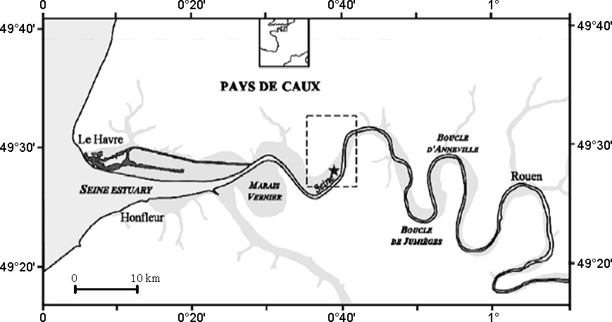
Location of the study site in the lower Seine Valley (Haute-Normandie, France), on the right bank of the Seine River [23].
Fig. 1. Localisation du site d’étude dans la basse vallée de la Seine (Haute-Normandie, France), sur la rive droite de la Seine [23].
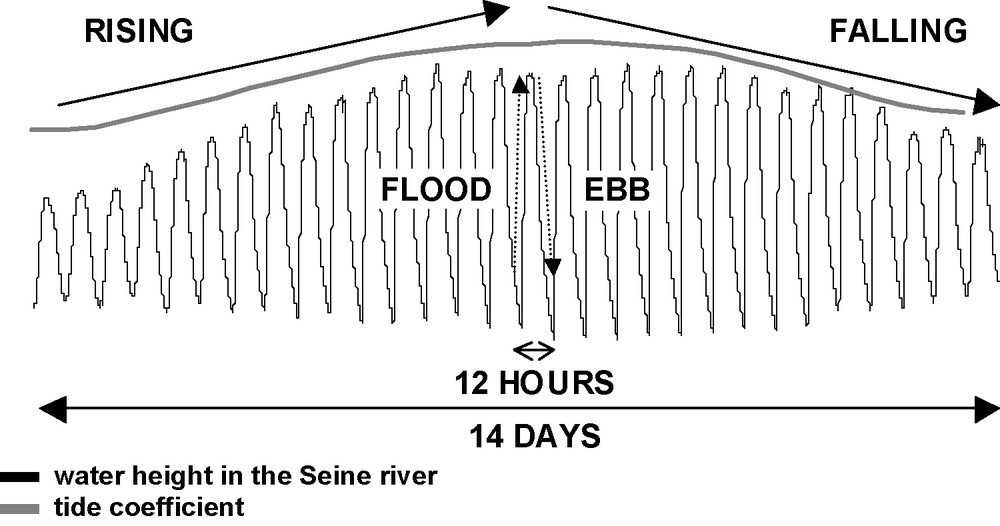
Seine River dynamics.
Fig. 2. Dynamique des hauteurs d’eau en Seine.
Bébec Creek drains a small catchment (about 10 km2) on the Pays de Caux plateau, and infiltrates into the swallow hole. Land use in the catchment consists of crops and grazing. Discharge in Bébec Creek varies from 3 l s−1 in summer dry periods to a maximum of 500 l s−1 in winter rainy periods. During these periods, the water in Bébec Creek is very turbid, up to 1666 NFU (1000 NTU).
The spring is located at the base of the plateau, at ‘Le Hannetot’, and is an overflow of the saturated zone. The Hannetot spring has been identified as the discharge point for water infiltrating via the swallow hole. Hannetot Spring discharge is composed of groundwater and the storm-derived water infiltrating via the swallow hole. After storms, turbidity at the spring can exceed 1000 NFU (600 NTU).
Data at the swallow hole and spring were collected continuously on a 15-min time interval using multi-parameter datasonds (6820 YSI), each comprising a turbidity probe, an electrical conductivity probe, and a pressure sensor. A rain gauge (ISCO 674) is located in the catchment. Discharge was measured at Hannetot Spring every 15 min (ISCO 4150 Doppler flowmeters).
The study of boundary conditions for this karst aquifer [7] demonstrates that the hydraulic gradient, which determines the flowpath within the aquifer, is governed by the difference between the piezometric level and the stage of the Seine River. The stage controls the drainage condition of the aquifer by the Seine. The aquifer is located in the estuarine part of the Seine River, i.e., it is influenced by tidal range. The Seine River thus is a prescribed head boundary condition that varies with the tide. Low stage in the Seine increases the hydraulic gradient and amplifies the drainage of the aquifer by the river, which may cause resuspension of intrakarstic sediment. High stage in the Seine decreases the hydraulic gradient and attenuates the drainage of the aquifer by the river, resulting in sedimentation of suspended matter within the karst-conduit network.
2.2 Frequency distribution decomposition (FDD)
Measurements of electrical conductivity and discharge have been used extensively to investigate the hydrodynamics of karst systems. Although the conductivity is not directly equivalent to concentrations of major ions, it has the advantage of being inexpensive and simple to measure, and time series at a very high resolution can be easily obtained. Conductivity is not a concentration, but rather is a general parameter that is correlated with the amount of total dissolved solids (TDS) in the water, and in karst systems is mainly controlled by calcium–carbonate equilibrium. Consequently, its variation in spring discharge reflects the varying contributions of different masses of water in the system under different types of flow conditions.
Bakalowicz [1,2] suggested that the different modalities of the conductivity frequency distribution (CFD) of karst spring discharge reflect the existence of geochemically distinct masses of water moving through the aquifer, which do not completely mix. The assumption is that the average conductivity of an individual water type depends on the spatial distribution of flow conditions. Bakalowicz used CFDs to classify the degree of karstification of different sites, associating the different modalities with the individual water types contributing to the spring, and suggesting that their number and spread represent the intensity of the karstification, or the efficiency of the karst conduit system. Other authors have used this qualitative approach to describe the karstification of other carbonate systems, for example the chalk of the northwestern Paris Basin [18] and the karst of the Grands Causses in southern France [26]. Massei et al. [24], expanding on the ideas proposed by Bakalowicz [1,2], showed that the frequency distribution of EC can be resolved quantitatively into the sum of two or more normally distributed populations, allowing the effective comparison of different CFDs. Further, they proposed that these populations represent distinct water types contributing to spring flow over a hydrologic cycle, and investigated the degree to which the various water types contribute to the total spring geochemistry. Here we apply this technique to both EC and D in the Norville karst system.
For EC and D, a histogram was constructed with the time series (EC or D) divided into 20 to 25 classes (Fig. 3). The histograms are replaced by their corresponding continuous distribution, which is afterwards decomposed into normally distributed components (populations) using a standard peak-fitting software program, such as PeakFit 4.0 (SPSS Inc.). Using the method of residues, all the modes constituting the original frequency distribution curve are identified, including previously hidden ones.
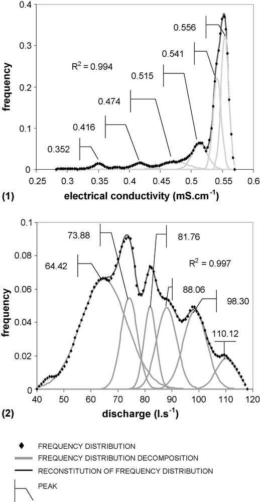
Frequency distribution decomposition (FDD) of electrical conductivity (1) and water discharge (2).
Fig. 3. Décomposition des distributions de fréquence de la conductivité électrique (1) et du débit (2).
The frequency distribution decomposition (FDD) defines the number and modes of the peaks. These peaks are interpreted as representing the normally distributed populations of conductivity or discharge values.
This method was not used with the turbidity frequency distribution, as most values were constrained within a very narrow range of turbidity (∼0 and 10 NFU) because of a constant base level. Therefore, the turbidity data set was divided into three groups according to their frequency distribution (Fig. 4).
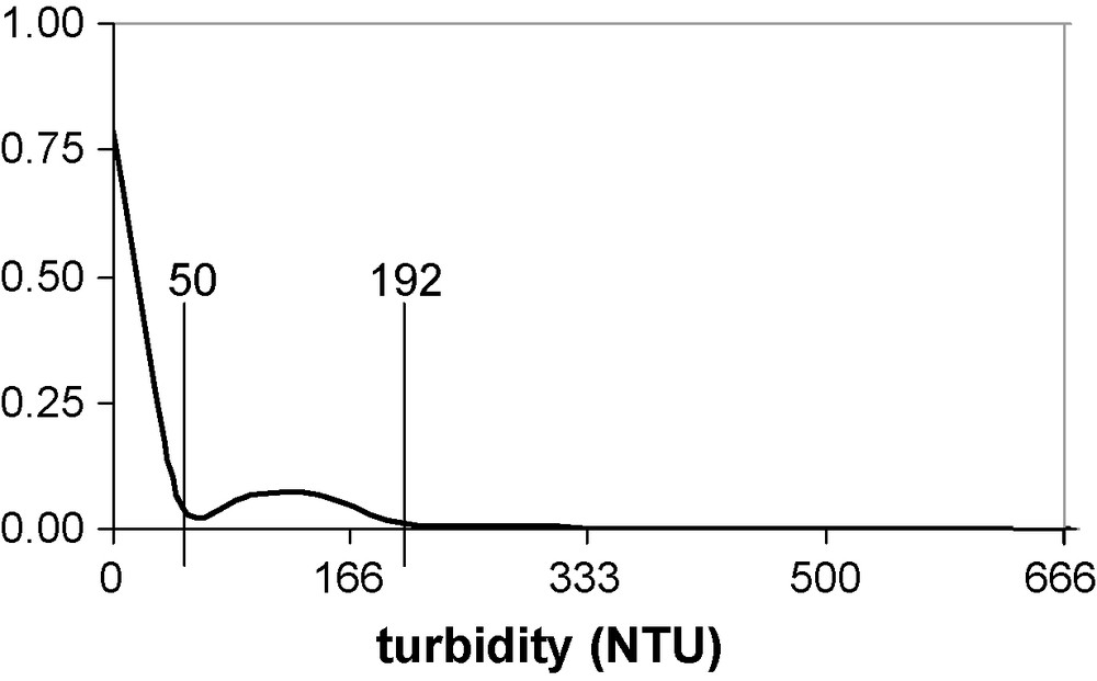
Frequency distribution of turbidity and the identified clusters ([0–50]; [50–192]; [192–666]).
Fig. 4. Distribution de fréquence de la turbidité et les groupes identifiés ([0–50] ; [50–192] ; [192–666]).
Massei et al. [24] show that within a single system, the CFD can take different forms, consistent on the one hand (the number of peaks), but varying on the other one (position and size of the peaks and distance between them). They therefore suggest that the type of karstic behaviour of a system can vary from one year to the next. In some hydrologic years, the different compartments contributing to flow are in better communication and more mixing occurs, resulting in peaks closer together. In other years, the compartments behave more independently and there is a greater difference in the water chemistries. Thus, unless averaged over many hydrologic years, the distance between the peaks cannot be taken as a single measure of karstic behaviour. The same processes can affect water discharge and turbidity. It is possible to compare the results obtained for different aquifers and different years. These results can be interpreted in terms of degree of karstification.
2.3 Univariate clustering
We used univariate clustering, with the XlStat (Addinsoft) software, to optimally partition observations in homogeneous clusters by minimization of intra-class inertia and maximisation of inter-class inertia, based on their description using a single quantitative variable. The Fisher algorithm guaranteed that the solution is the best that can be obtained [6]. The results of FDD were used to define the number of classes for the univariate clustering of EC and D data sets. For example, the FDD of D and EC (Fig. 3) shows six classes. We therefore made a univariate clustering of the D data set with six classes. Table 1 shows that the results obtained by the FDD are close to those obtained by univariate clustering, with a percentage of variation of less than 5%.
Comparison of the results obtained by univariate clustering and FDD for water discharge and electrical conductivity data sets; % = percentage of variation
Tableau 1 Comparaison des résultats obtenus par le partitionnement univarié et la décomposition des distributions de fréquence pour les données de débit et conductivité électrique ; % = pourcentage de variation
| Class | Barycenter from univariate clustering | Peak mode from FDD | % |
| Water discharge (l s−1) | |||
| 1 | 63.98 | 64.42 | 0.7 |
| 2 | 72.75 | 73.88 | 1.5 |
| 3 | 80.29 | 81.76 | 1.8 |
| 4 | 89.47 | 88.06 | 1.6 |
| 5 | 11.90 | 98.30 | 3.7 |
| 6 | 112.03 | 110.12 | 1.7 |
| Electrical conductivity (μS cm−1) | |||
| 1 | 345 | 352 | 2.0 |
| 2 | 417 | 416 | 0.2 |
| 3 | 469 | 474 | 1.1 |
| 4 | 513 | 515 | 0.4 |
| 5 | 545 | 541 | 0.7 |
| 6 | 557 | 556 | 0.2 |
3 Results and discussion
3.1 Typology of water masses
In binary karst systems, groundwater is more mineralized than surface water. A decrease in EC indicates the arrival of surface water. Increasing turbidity indicates either the arrival of surface water or the resuspension or erosion of intrakarstic sediments [8,19,22,29,30] (Table 2). The understanding of transport properties is investigated here using the relations between EC, T, and D. The hydrologic processes corresponding to each water type are interpreted by comparing the range of EC, T and D represented by each population. For each variable, three modalities are defined:
- • low values of EC or D: association of the first and the second peaks obtained by the FDD for each variable (Fig. 3), and low turbidity (T) values (first cluster, Fig. 4);
- • mean values of EC or D: association of the third and the fourth peaks (Fig. 3), and mean T values (second cluster, Fig. 4);
- • high values of EC or D: association of the fifth and the sixth peaks (Fig. 3), and high T values (third cluster, Fig. 4).
Identification of transport properties according to electrical conductivity and turbidity variations
Tableau 2 Identification des propriétés de transport selon les variations de conductivité électrique et la turbidité
| Electrical Conductivity | |
| weak or mean values → surface water | strong values → groundwater |
| Turbidity | |
| weak values | |
| deposition of suspended matter | direct transfer of groundwater |
| mean or strong values | |
| direct transfer of surface water | resuspension of intrakarstic sediments |
By combining these three modalities for the three variables, we obtained 27 theoretical combinations, only 18 of which being hydrologically meaningful based on the values of the three variables (Table 3). Based on these combinations, we can identify the transport properties/modalities and their periods of occurrence in the annual cycle (Fig. 5). In brief, at any time, the combinations allow identification of the transport properties of the system during any flood considered throughout the entire annual cycle. From these results, the proportion of the different water masses can be calculated by multiplying the water discharge values by the time during which the transport modalities of the water mass fall into each category. Table 4 shows that the annual volume of spring water is decomposed into 47.7% of groundwater, 23.7% of surface storm-derived water accompanied by direct transfer of particles, and 28.6% of water that is associated either with deposition (13.2%) or resuspension (15.4%) of intrakarstic sediment. Periods of deposition are associated with turbid floods (i.e., a high contribution of surface water). Resuspension periods can be associated either with surface water (flushing effect/pressure-pulse transfer) or with groundwater (the re-filling of the conduit network after the evacuation of surface water). However, it is possible to distinguish readily between these respective contributions by focusing on selected events within the annual graph obtained from univariate clustering. For the annual cycle studied, depositional periods occur mainly from February to May, whereas resuspension usually takes place from June to August (Fig. 5).
Theoretical combinations and their hydrological meaning
Tableau 3 Combinaisons théoriques et leur signification hydrologique
| EC | D | T | Hydrological meaning |
| weak | weak | weak | none |
| weak | weak | mean | none |
| weak | weak | strong | none |
| weak | mean | weak | deposition of suspended matter |
| weak | mean | mean | direct transfer of surface water |
| weak | mean | strong | direct transfer of surface water |
| weak | strong | weak | none |
| weak | strong | mean | direct transfer of surface water |
| weak | strong | strong | direct transfer of surface water |
| mean | weak | weak | deposition of suspended matter |
| mean | weak | mean | direct transfer of surface water |
| mean | weak | strong | none |
| mean | mean | weak | deposition of suspended matter |
| mean | mean | mean | direct transfer of surface water |
| mean | mean | strong | none |
| mean | strong | weak | direct transfer of surface water |
| mean | strong | mean | direct transfer of surface water |
| mean | strong | strong | direct transfer of surface water |
| strong | weak | weak | direct transfer of groundwater |
| strong | weak | mean | resuspension of intrakarstic sediments |
| strong | weak | strong | none |
| strong | mean | weak | direct transfer of groundwater |
| strong | mean | mean | resuspension of intrakarstic sediments |
| strong | mean | strong | none |
| strong | strong | weak | direct transfer of groundwater |
| strong | strong | mean | resuspension of intrakarstic sediments |
| strong | strong | strong | none |
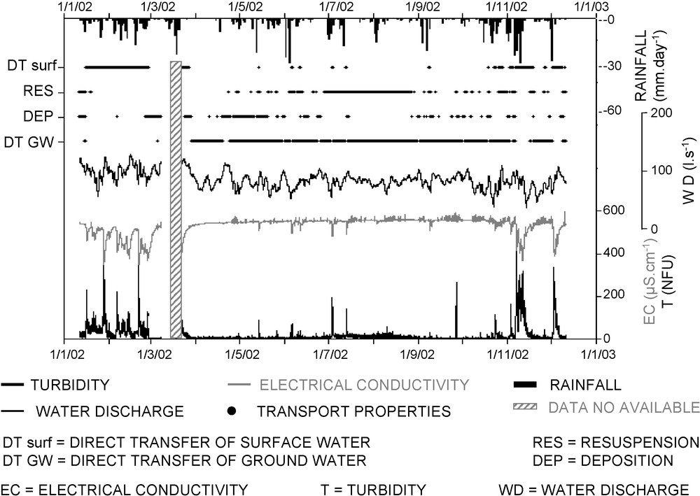
Transport properties and their occurrence periods at the Hannetot karst spring from January to December 2002.
Fig. 5. Propriétés de transport et leurs périodes d’occurrence à la source karstique du Hannetot de janvier à décembre 2002.
Percentage of annual volume of water masses
Tableau 4 Pourcentage en volume annuel des masses d’eau
| Transport properties | % of annual volume |
| Deposition of suspended matter | 13.2 |
| Direct transfer of surface water | 23.7 |
| Direct transfer of groundwater | 47.7 |
| Resuspension of intrakarstic sediments | 15.4 |
| 100.0 |
3.2 Comparison between univariate clustering and normalized EC–T curve
Many authors [8,9,25,28,31] have shown that it was possible to characterize the transport properties of a river by studying the relationships between the sediment concentration and the flow during the rain events. Valdes et al. [29,30] applied the method of Williams [31] to the field of karst hydrology using EC–T relationships. The analysis of EC–T relationships results in improved understanding of dissolved and suspended solids transport in response to rain events by highlighting the hydrosedimentary processes: direct transport, resuspension of intrakarstic sediments, or deposition of suspended matter. This method appears suitable for the study of EC, T and D relationships at the flood scale [3,8,19]. Here, it was used to compare the results with those obtained by univariate clustering to check the similarity of the results offered by the two methods, as well as their respective accuracy.
Two examples have been chosen, the first in March and the second in May (Fig. 6). Flood events were decomposed into several parts (indicated by different letters), each characterizing a transport modality (Fig. 6); the same data sets were then used to describe EC–T curves, where the same parts are indicated by the same letters as in Fig. 7. For these examples, the same results are obtained using the method of normalized EC–T curves and that of univariate clustering (Table 5). Thus, at the scale of the event, the study of annual data sets by univariate clustering provides the same results and the same accuracy as those obtained by the normalized EC–T curve, with the advantage of determining transport modalities concurrently for the entire annual period.
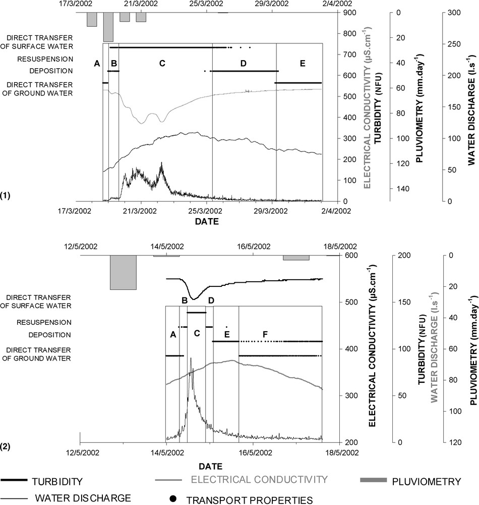
Two examples of univariate clustering results at the scale of a flood event ((1): March 2002 and (2): May 2002); letters represent parts of hydrograph with different transport properties identified by univariate clustering.
Fig. 6. Deux exemples de résultats du partitionnement univarié à l’échelle de la crue ((1) : mars 2002 et (2) : mai 2002) ; les lettres représentent les parties de l’hydrographe, avec différentes propriétés de transport, identifiées par le partitionnement univarié.
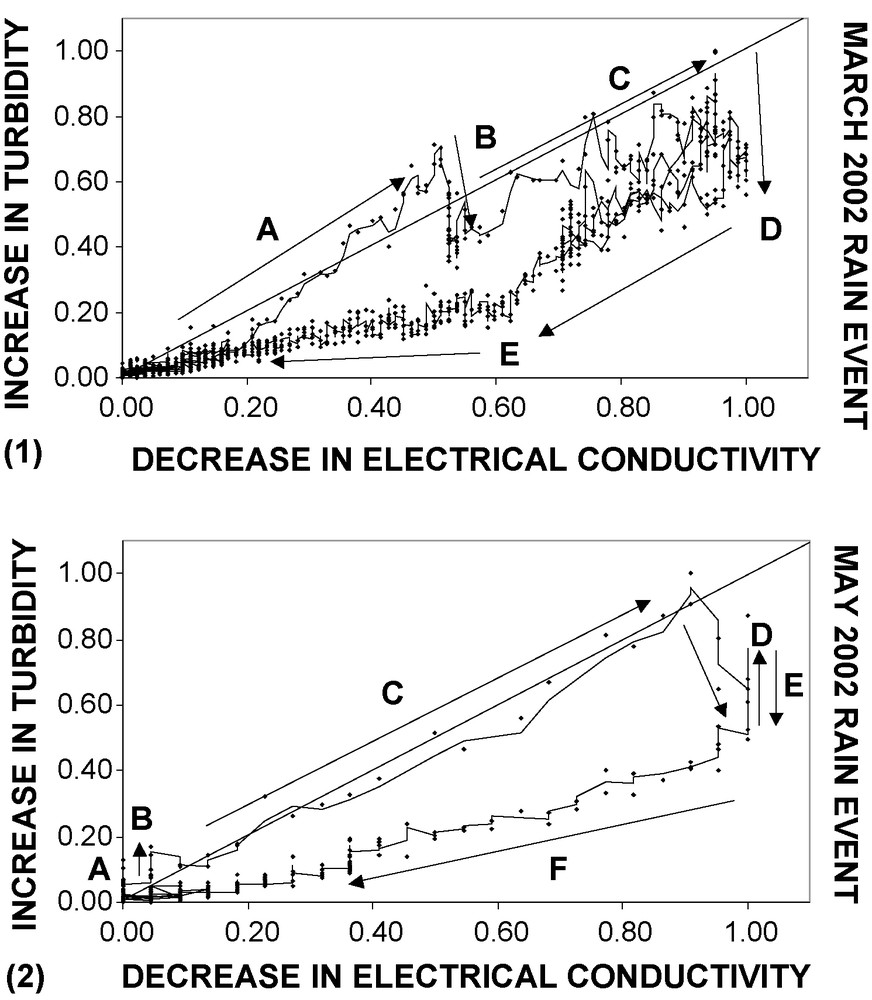
Normalized EC–T curves during two flood events ((1): March 2002 and (2): May 2002); letters represent parts of hysteresis curve with different transport properties identified by observation of the mean slopes.
Fig. 7. Courbes conductivité électrique–turbidité normalisées durant deux épisodes pluvieux ((1) : mars 2002 et (2) : mai 2002) ; les lettres représentent les parties de la courbe d’hystérésis, avec différentes propriétés de transport identifiées par l’observation des pentes moyennes.
Comparison of the results obtained by normalized electrical conductivity–turbidity curves and univariate clustering
Tableau 5 Comparaison des résultats obtenus par les courbes de conductivité électrique–turbidité normalisées et le partitionnement univarié
| Results obtained by | |||
| Date | Part | Normalized EC–T curve | Univariate clustering |
| March 2002 | A | α = 1: direct transfer | direct transfer |
| B | α < 1: deposition | deposition | |
| C | α = 1: direct transfer | direct transfer | |
| D | α < 1: deposition | deposition | |
| E | α = 1: direct transfer | ||
| May 2002 | A | α = 1: direct transfer | direct transfer |
| B | α > 1: resuspension | resuspension | |
| C | α = 1: direct transfer | direct transfer | |
| D | α > 1: resuspension | resuspension | |
| E | α < 1: deposition | deposition | |
| F | α = 1: direct transfer | direct transfer |
3.3 Response of the karst system
Fig. 5 shows that during the low-water period (June to August), the spring is vulnerable to turbid floods resulting from resuspension of intrakarstic sediments. Given the absence of any rain events, the cause of the resuspension cannot be the infiltration of storm-derived water at the swallow hole. Resuspension therefore must result from increasing spring discharge related to an overall increase of the hydraulic gradient in the aquifer (the combined effect of tidal range and natural Seine River discharge).
Fig. 8 shows that the deposition periods from February to May occur during high water discharge in the Seine River and that resuspension periods from June to August occur during low-water discharge. This demonstrates the importance of the prescribed head boundary condition defined by the Seine River, which changes during the hydrological annual cycle.
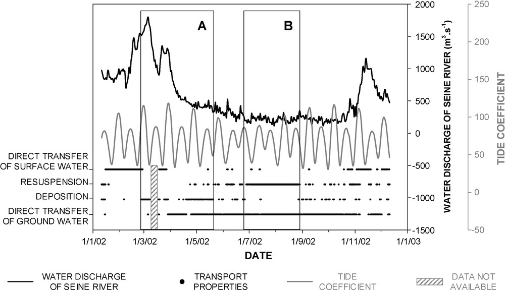
Transport properties and Seine River dynamics (water discharge and tide coefficient); the depositional period, from February to May (A), occurs during higher water discharge of the Seine River, and the resuspension period, from June to August (B), occurs during lower water discharge of the Seine River.
Fig. 8. Propriétés de transport et dynamique de la Seine (débit et coefficient de marée) ; les périodes de dépôt, de février à mai, ont lieu durant les plus forts débits de la Seine, et les périodes de remise en suspension, de juin à août, ont lieu durant les plus faibles débits de la Seine.
4 Conclusion
The univariate clustering method applied to high-frequency time series of electrical conductivity, turbidity and water discharge allows the identification of the various modes of transport and their occurrence periods during the annual hydrologic cycle. This method, based on the annual data sets, offers the same results as those obtained by normalized EC–T curve at the flood scale. Moreover, this method allows calculation of annual water masses. The results show that the annual volume of spring water is composed of 47.7% of groundwater, 23.7% of surface storm-derived water accompanied by the direct transfer of particles, and 28.6% of water, which is associated either with deposition (13.2%) or with resuspension (15.4%) of intrakarstic sediment. Release of groundwater occurs during low-water periods and release of floodwater occurs during winter recharge and storm events in summer. The release of spring water associated with particle deposition occurs during low-intensity rain events from February to May, when the Seine River discharge is high. The release of spring water associated with resuspension occurs from June to August, when the Seine River discharge is low.