

Version française abrégée
Le but de cet article est de présenter les premiers résultats d’une campagne d’étude des effets de charge océanique, menée dans le Nord-Ouest de la France, à l’aide de diverses techniques géodésiques. La comparaison des observations avec les valeurs théoriques permet de valider les modèles de marée et d’estimer le bilan d’erreur pour chaque instrument.
Une première campagne d’observation en gravimétrie absolue, réalisée à Brest en mars 1998, avait mis en évidence des écarts de 16 % entre les effets de charge océanique observés et les effets prédits [18]. Trois jours de données GPS sur la même région [29] nous avaient confirmé la nécessité d’une campagne de plus grande envergure, sur une plus longue durée.
Nous montrons ici des observations gravimétriques (relatives et absolues), inclinométriques – pendules de Blum [27] – de stations GPS et, pour la première fois, avec l’objectif d’observer les effets de charge océaniques, des observations de la Station laser ultra mobile (FTLRS, voir [24]). Les mesures ont été faites sur différents sites répartis entre Brest et Cherbourg, entre le 12 et le 19 mai 2004 – sauf la FTLRS, qui a fonctionné pendant les mois de septembre et d’octobre 2004. Dans chaque cas, les effets de charge océanique ont été calculés à partir des huit ondes principales du modèle de marée FES2004 [20], en utilisant le formalisme classique décrit par Farrell [11].
Des récepteurs GPS – prêtés par l’Insu – ont été installés temporairement sur la zone d’étude, en complément des stations permanentes du RGP (Fig. 1). Les résultats ont été obtenus à l’aide du logiciel GAMIT 10.1 [16]. Nous avons utilisé des paramètres de traitement classiques : sessions de 2 h, orbites IGS, angle de coupure de 10°, délais atmosphériques estimés toutes les 30 min. La mise en référence est assurée par une contrainte sur la position de 10 stations IGS du réseau de référence IGS00 [12]. La comparaison des données aux effets de charge océanique prédits montre un bon accord (Fig. 2).
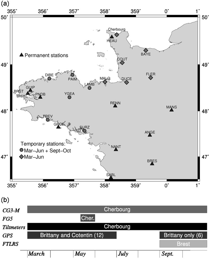
(a) Map of northwestern France, showing the different locations of the GPS receivers during the campaign. (b) Several techniques have been used for this study, with different recording periods. The text inside the bars indicates the instrument locations. For interpretation of the references to colour, see the web version of this article.
Fig. 1. (a) Carte du Nord-Ouest de la France, montrant les emplacements des récepteurs GPS utilisés pendant la campagne. (b) Plusieurs techniques ont été mise en œuvre pour cette étude, ayant chacune leur propre période d’observation. Le texte à l’intérieur des barres indique le lieu d’installation. Pour les indications de couleur, voir la version électronique de cet article.
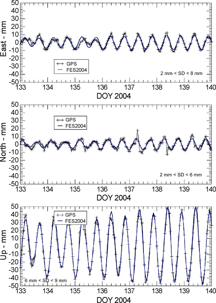
GPS loading observations at Brest plotted with black crosses plus black curve, between day 133 and 140 of year 2004 (12 to 19 May) for the east, north and up components (the range for standard deviation (SD) is also given). Loading computation for FES2004 (blue curve) is superimposed. Units are in millimetres. For interpretation of the references to colour, see the web version of this article.
Fig. 2. Mesures GPS de l’effet de charge océanique à Brest (croix et courbe noires), entre les jours 133 et 140 de 2004 (du 12 au 19 mai) pour les composantes est, nord et verticale (l’écart type des mesures – noté SD – est donné en bas du graphique). L’effet de charge calculé avec le modèle de marée FES2004 est tracé en bleu. Les unités sont des millimètres. Pour les indications de couleur, voir la version électronique de cet article.
À Cherbourg, nous avons choisi un site souterrain de l’armée, lieu calme et thermiquement stable, pour installer les inclinomètres. Le gravimètre absolu FG5 et un gravimètre relatif Scintrex CG-3M ont été co-localisés sur ce site. Après avoir appliqué les corrections classiques aux variations de gravité – marées terrestres, effet du pôle, atmosphère –, le signal résiduel donne l’effet de charge océanique observé. On peut le comparer au signal prédit (Figs. 3 et 4) et voir l’excellente corrélation entre les deux. L’écart en amplitude est inférieur à 7 %, ce qui est meilleur que lors de la première campagne en Bretagne.
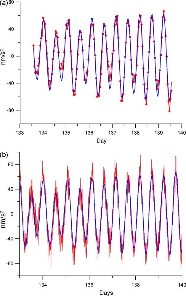
(a) Absolute gravity measurements of ocean loading at Cherbourg (red curve and dots), plotted with the predicted signal computed from FES2004 (blue curve). The number of days in 2004 is given as the abscissa, spanning from 12 to 19 May 2004. Units are in nm/s2. (b) Same as (a), but for Scintrex CG3-M gravity measurements (red curve) with the predicted signal (blue curve), at Cherbourg. For interpretation of the references to colour, see the web version of this article.
Fig. 3. (a) Effet de charge océanique mesuré par gravimétrie absolue à Cherbourg (courbe et points rouges). Le signal théorique calculé avec le modèle FES2004 est en bleu. Les abscisses sont en numéro de jour pour l’année 2004, et les signaux sont en nm/s2. (b) Même chose, pour des observations du Scintrex CG3-M (courbe rouge) et le signal prédit correspondant (courbe bleue), toujours à Cherbourg. Pour les indications de couleur, voir la version électronique de cet article.
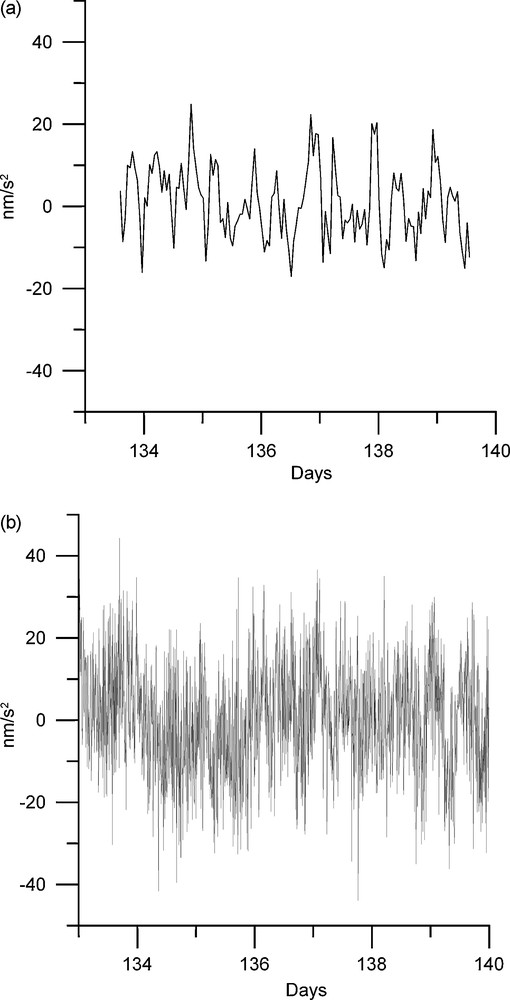
(a) Gravimetric residues computed between the FG5 signal and the predicted one. In fact, they are the differences between the two curves, red and blue, of Fig. 3. (b) Same as (a), but for the Scintrex data. For interpretation of the references to colour, see the web version of this article.
Fig. 4. (a) Résidus calculés à partir des observations de gravimétrie absolue (FG5) et des effets de charge prédits. Il s’agit simplement de la différence entre les courbes rouge et bleue de la Fig. 3. (b) Même chose avec les observations de gravimétrie relative (Scintrex CG3-M). Pour les indications de couleur, voir la version électronique de cet article.
L’inclinomètre montre aussi un très bon accord entre effet observé et prédit (Fig. 5). Le rapport signal/bruit est excellent – estimé à environ 0.005 μrad, et c’est la seule méthode pour laquelle l’effet de charge océanique est supérieur à la marée terrestre.
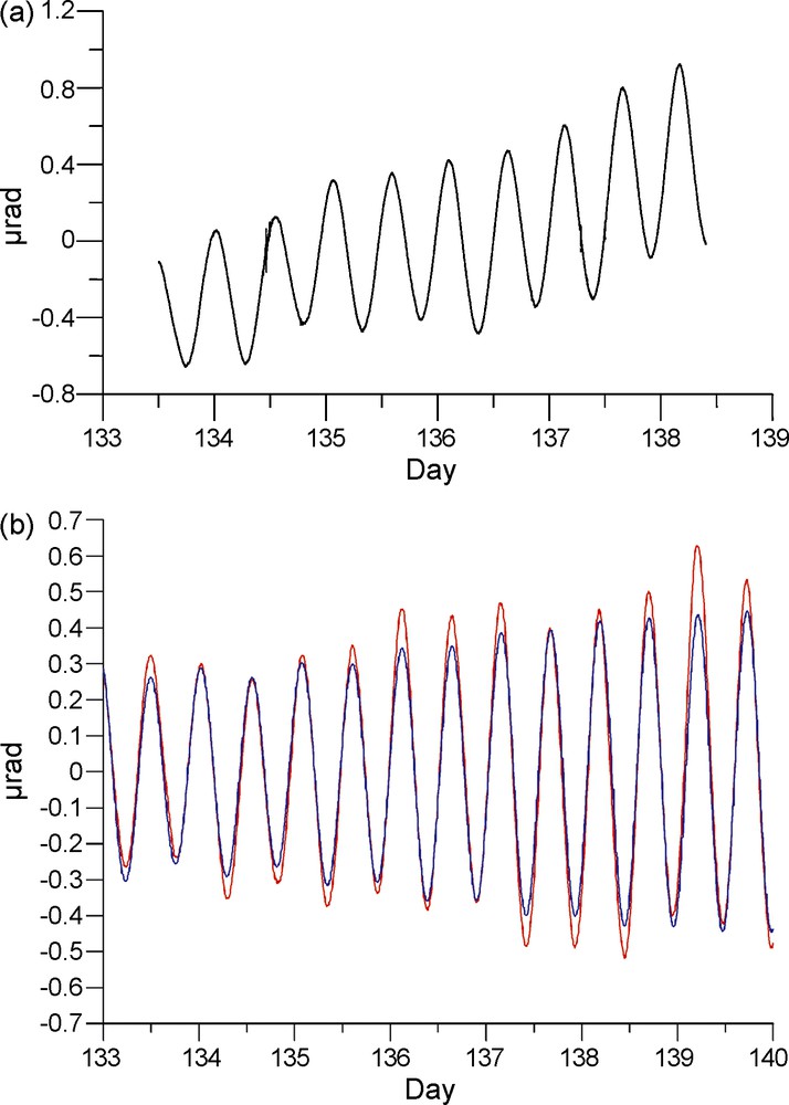
East–west tilt observations from silica pendulum tiltmeter at Cherbourg, during the same period as gravimetric plots: (a) raw signal, (b) signal corrected from all constituents, except loading tide (red curve), and predicted curve using FES2004 tide model (blue curve). Units are in microradians. For interpretation of the references to colour, see the web version of this article.
Fig. 5. Observations inclinométriques dans la direction est–ouest à partir d’un pendule horizontal en silice, faites à Cherbourg pendant la même période : (a) signal brut, (b) signal corrigé de tous les effets connus, excepté l’effet de charge océanique (courbe rouge) ; la courbe prédite à partir du modèle de marée FES2004 est en bleu. Les unités sont des microradians. Pour les indications de couleur, voir la version électronique de cet article.
Finalement, malgré la ténacité des opérateurs et à cause des conditions météorologiques, la FTLRS n’a pu observer que ponctuellement, pendant une période de deux mois. La comparaison des mesures avec la courbe prédite (Fig. 6) montre qu’il aurait fallu une série de points au moins toutes les six heures pour pouvoir suivre le signal temporel, ce qui n’a pas été possible. On a quand même pu ajuster aux données l’amplitude de l’onde principale M2, et obtenir un résultat de 3,731 cm, très proche des 3,730 cm de l’onde théorique.
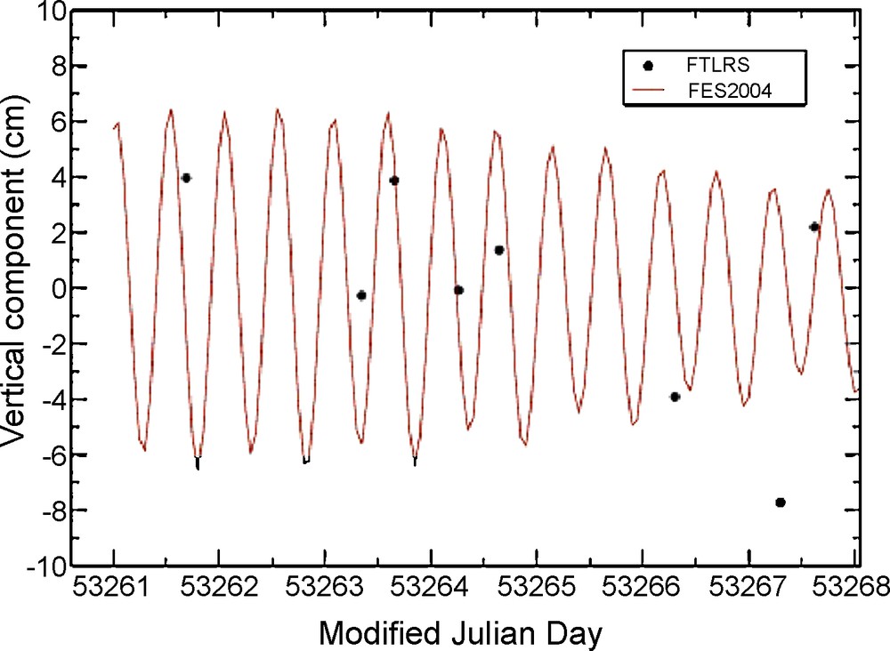
Zoom over seven days of observation during the FTLRS operation. Black dots are vertical coordinates of the station computed every 6 h. The load vertical displacement from M2 wave is plotted in red. For interpretation of the references to colour, see the web version of this article.
Fig. 6. Extrait de sept jours de mesures réalisés pendant la période d’observation avec la FTLRS. Les coordonnées verticales calculées toutes les 6 h sont représentées par des points noirs. Le déplacement vertical sous la charge de la marée est la courbe rouge. Pour les indications de couleur, voir la version électronique de cet article.
Ces premiers résultats mettent en évidence la très bonne qualité des données récoltées par les différents appareils. Ils valident l’utilisation du modèle de marée FES2004, qui améliore la prédiction des effets de charge dans cette zone.
1 Introduction
We present here the first results from a field campaign dedicated to the observation of the ocean tide loading. Several geodetic techniques were used together in the same zone (northwestern part of France), during the same period. The aim of this paper is to validate the capability of each technique to characterize the ocean loading effect. We also compare the various observations to loading predictions computed using one of the most recent ocean tide models (FES2004, [20]), and estimate the residual values. This preliminary paper presents an overview of the whole campaign, with all of the datasets. More detailed papers focusing on one particular technique will follow later.
Loading effects are much stronger in the vicinity of the coasts, where ocean tides are amplified by strong bathymetric variations and by short-wavelength geometric features of the coastline. It is especially true in some sectors, such as the Bay of Fundy (Canada), where tidal ranges can reach 16 m and in the Bay of Mont St Michel, located between Cotentin and Brittany (see Fig. 1a), with peak-to-peak tidal ranges up to 14 m. Our study focuses on a large area in this Brittany region to install the different instruments.
For the first campaign in March 1998, an absolute gravimeter was installed during four days a on the headland of Brittany (at Brest). There was a good temporal correlation between the predicted model of ocean tide loading and the observations [18]. We found no phase shift between these signals; however, we detected a 16% discrepancy between the amplitudes of the model and the observations. Some improvements may be expected by applying more advanced ocean tide models, with higher-resolution ocean grids, through a better determination of the coastline, or through a better Earth model used for the Green functions, etc. [5]. Several available ocean tide models have been tested. We found only 6% RMS discrepancy between the estimated loading effects, but a systematic bias with the observations persisted. This bias depends on the geographical location and on the geodetic parameter taken into consideration. One year later, we attempted to use three days of GPS records at Brest to determine loading displacements [29]. We concluded that longer observations are required to obtain accurate enough positions of the station.
These preliminary results needed to be continued, so we organized a more ambitious campaign in Brittany and Cotentin (Fig. 1a). This operation involved several techniques: relative and absolute gravimeters, Blum-like tiltmeters [27], GPS, and French Transportable Laser Ranging Station (hereafter FTLRS, see [24]). They were installed at several sites: Brest and Cherbourg gathered more than one technique, and GPS receivers were distributed over a large area between these two cities. Fig. 1a shows the location of each instrument used in our study. Relative gravimeters and inclinometers provided measurements for more than one year from March 2004; GPS receivers were installed at the same time, but only for a four-month duration, and the absolute gravimeter worked during seven days in this period. A second GPS campaign was carried out in September and October 2004 when the FTLRS was in Brest (see Fig. 1b for more details).
Several research groups were involved in planning, installing, and maintaining all instruments, in analysing the various datasets and finally in interpreting the results. The FTLRS was the most difficult technique to manage from a logistical viewpoint. Autumn is also not the best season of the year for a technique that needs a cloudless sky, but some results have been obtained and we can present here the first experiment of laser ranging dedicated to ocean loading.
In this paper, we focus on the period where most of the techniques were operating at the same time. The period spans from 12 to 19 May 2004, and all available instruments were in field operation, except for the FTLRS, which functioned only four months later. We first present each technique separately. The long duration gravimetric and tilt signals will be analysed in a further work, jointly with instrumental cross-comparison.
2 Computation of ocean loading
We used FES2004 [20], one of the most recent ocean tide models available. It is based on the same hydrodynamical scheme as FES2002, but it assimilates more satellite and tide gauge data. Both models are computed on the same finite element grid [17]. We use a version interpolated onto a regular rectangular grid of 1/8 degree. This corresponds to cells of 13.8 km by 9.3 km at the latitude of our study. A lot of tidal constituents are available: 12 in the semidiurnal band, 14 in the diurnal band, 8 for long periods and one quarter diurnal. We limit our study to the diurnal and semidiurnal periods and, among them, to the eight main tidal constituents, M2, S2, K1, O1, N2, P1, K2, and Q1, whose combination provides most of the tidal amplitude in our region, which will be verified with the observations presented here.
Ocean tide loading causes several effects: Newtonian attraction, deformation under the load, and perturbation of the gravity potential (due to mass redistribution associated with deformation). These effects have a linear dependence on the load. They can be computed using a formalism based on a given ocean tidal model, plus an appropriate Green's function (one specific function for each observed parameter). A complete description of the method is given in [11] or [26]. The Green's functions at a given location can be computed using the following linear relations:
| (1) |
| (2) |
| (3) |
| (4) |
| (5) |
3 GPS experiment
GPS is well suited to monitoring 3D positioning variations. This space geodesy technique is easy to set up and relatively low-cost, and allows a dense cover of the studied area. A GPS network allows us to detect spatial variations of the discrepancies between the data and he geodynamical models. In addition to the local permanent GPS stations of the global French GPS permanent network (RGP [http://geodesie.ign.fr/RGP/index.htm]), a set of GPS receivers was temporarily installed in a large area surrounding the Mont St Michel Bay (Fig. 1a). These dual-frequency receivers (provided by the ‘Institut national des sciences de l’Univers’ and the ‘Laboratoire Dynamique de la lithosphère’) were equipped with choke-ring antennas and recorded every 30 s both code pseudo-range and carrier-phase measurements. The GPS experiment was divided into two periods (cf. Fig. 1b). During the first period, from March to June 2004, 12 GPS receivers were temporarily installed in Brittany and Cotentin. The second period, from September to October 2004, coincided with the autumnal equinox tides. For this period, in addition to the FTLRS station located at Brest, six GPS receivers were temporarily re-installed in Brittany, where the tidal phenomenon has the highest amplitude, particularly in its vertical component.
The results we present here were obtained using the GAMIT 10.1 software [16], although some tests have been performed with the Bernese software version 4.2 [15] and GIPSY OASIS II [30]. We processed a regional network including the campaign sites and 10 European IGS stations from the IGS00 reference network [12] in order to determine the reference frame. The amplitude of the Ocean Tide Loading effect reaches up to 8 cm in the vertical component (for instance at Brest) with a main semi-diurnal period. We therefore used two-hour sessions every hour (best trade off between accuracy and sampling of the displacements). The GPS processing parameters we used are quite classical: IGS precise orbits, IERS Bulletin B EOPs, 10° cut-off angle; atmospheric delays were estimated every 30 min using the Niell [25] mapping functions. The reference frame realisation within the GPS analysis was ensured by tightly constraining the IGS stations to their IGb00 positions, including OTL effects from the FES2004 model [17,20]. We previously performed a free network processing to obtain a priori positions for the campaign stations, to which we added OTL FES2004 effects. Constraints on these fitted a priori positions were kept to the centimetre level. Alternative strategies (different types of constraints and a priori positions, a posteriori 7-parameter transformation) have been tested and lead to similar results. Standard deviations on the GPS positions range from 2 to 6 mm on the N component, 2 to 8 mm on the E component and 6 to 9 mm on the U component, respectively. This is consistent with what we can expect from this kind of processing with short sessions and a regional network.
Preliminary time series of 3D GPS station positions (see Fig. 2) are compared with the FES2004 tidal model. The agreement is generally very good: mean RMS between GPS and FES2004 positions are 2.5, 3.1 and 4.5 mm for East, North and Up components respectively (on an 8-day time series, all campaign stations). Amplitudes are also in good agreement for the three coordinate components. Only a few phase shifts are observed in the data (e.g., day 135 at BRST). They do not cover the whole network and could be due to interesting local effects. We look forward to processing longer time series in [28] and in [22].
4 Gravimetric experiments
The first campaign, in March 1998, showed that precise tidal gravity measurements can provide a high-quality study of ocean tide loading. A FG5 absolute gravimeter recorded the time variations during six days. It allowed us to validate the ocean tide models in the diurnal and semi-diurnal frequency bands. However, the 16% discrepancy between observations and the predicted loading highlighted the limit in accuracy of our knowledge about this phenomenon. Others studies used relative gravity measurements as a tool to estimate the performances of tidal models [1,4,7]. The gravimetric residuals may be reduced by a better refinement of the tide grid, using for example a local ocean tide model in the vicinity of the gravimetric station, or taking into account for the non-linear part of the signal.
A FG5 absolute gravimeter had been installed in Cherbourg, from 12 to 19 May 2004, recording gravity measurements each hour (northwestern France, see Fig. 1). In this sector, ocean tides can reach up to 7 m in amplitude. Our aim is to observe ocean tide loading in a hydrodynamic context quite different from the one of Brest, already studied in the previous campaign. Moreover, as the bay of Mount St Michel is located 140 km southward, we expected to observe interesting signals, such as non-linear constituents. They have been already suggested by [8] or [13] as impacting on inland superconducting gravimeters.
The usual corrections for body tides, polar effect and atmospheric loading corrections were applied to the gravimetric data. Fig. 3a shows the observed gravity signal, jointly with the predicted ocean tide loading. There is a good agreement between the two curves, even if the observations seem to be sometimes lower than the computations. The explanation may be due to the 1-h sampling rate, which can sometimes truncate the extreme values of the phenomenon. We found a linear regression coefficient of 0.934. That indicates a real improvement in the computations obtained with the eight main tidal constituents of FES2004. The gravimetric residuals calculated as the difference between the observed and the predicted signals have a RMS of only 9 nm/s2.
Since March 2004, a spring gravimeter, CG3-M type, has also been installed at Cherbourg, close to the FG5. We present here the observations recorded during the common measurement period (day 133 to 140 of year 2004). The body tide was computed with Eterna software [31] using the Hartmann and Wenzel tidal potential [14]. For the atmosphere, we used the European Centre for Medium-range Weather Forecasts (ECMWF) data set at 3-h sampling, and the computation is based on the inverted barometer hypothesis with an ocean/continent function gridded at 0.1 degree (see [6]). This atmospheric loading estimation is more accurate than the classical pressure correction obtained by applying a multiplicative factor to the local pressure [6]. With a higher sampling rate of 5 min, the relative gravimetric observations look noisier (Fig. 3b), but this is not relevant and the linear regression coefficient computed without filtering the data is 1.013. The observed signal is in excellent agreement with the predicted one, and the RMS of the residuals reaches 13 nm/s2, which is smaller than the instrumental precision estimated at 50 nm/s2. Fig. 4a and b shows the gravimetric residues computed for the absolute and relative observations.
High-precision microgravimetric studies are always a useful tool to validate tidal models and loading theory in coastal regions. The actual residuals are very small, and the remaining noise comes from the instrumental measurements, from the applied corrections (such as the atmospheric loading), from other environmental features such as higher (or lower) sea tidal height due to weather conditions, or even, from the predicted loading.
5 Tilt experiment
Inclinometry is a high-performance tool, and probably the most sensitive and least expensive one for studying ocean tide loading deformation near the coast (e.g., [21,23]). It consists in measuring the angular time variation between the normal to the instant geoid (plumb line or local vertical) and an initial state of this direction. The instruments devoted to this kind of measurement can resolve up to 10–9 rad (with a compact Blum's pendulum based on a Zöllner suspension beam, [3,27]) or even 10–10 rad (using a long hydrostatic tiltmeter, see, e.g., [2]).
Although hydrostatic devices show better long-term behaviour (less drift), smaller temperature dependence and better sensitivity, they must be installed in unperturbed, long (say > 30 m) and horizontal tunnels, which is not feasible everywhere in our study area. For our study, we installed two Blum's pendulums in the north–south and east–west directions, in an underground depository in Cherbourg (France).
The appropriate Green's function provides, by convolution, the tilt response to the load. An important property of this Green's function is that it behaves like 1/r2, r being the distance to the point load. This leads to an invariance of scale: a 1-kg load at 1 m produces (more or less, depending on the Earth model) the same tilt as 1 tonne at 1 km and so on. In the framework of our study, this confers a higher dependence on the closest loads with respect to gravity or displacement responses.
The pendulum signals have been recorded using a 22-bit ADC at a 30-s initial sampling rate, from March 2004 to July 2005. Two steps have been addressed to ensure the calibration. Firstly, an electronic calibration is made in the laboratory, to determine the voltage response to a displacement of the beam. Secondly, the mechanical gain of the tiltmeter-pendulum is derived from its eigenperiod, which is adjusted when the pendulum is settled. We estimated that a final accuracy of a few percent is hard to reach and actually consider that 5% is realistic. This limitation complicates the comparison between models and records. A procedure that uses the ratio between waves may be more suitable than the direct comparisons reported here.
The extract of the raw data presented in Fig. 5a shows a clear tidal signal. The seismic noise level is very low, confirming that the tunnel is a quiet place, with very few temperature fluctuations. To compare the observations with the ocean tide loading prediction, we first remove the theoretical Earth tide contribution as provided by the ETERNA package, involving a Wahr–Dehant model [10]. The comparison between the EW de-tided observations (red curve) and ocean tide loading predictions (blue curve) can be seen in Fig. 5b. To make this plot, tilt data have been decimated to a 5-min sampling rate. The agreement between the two curves is quite good, with no phase shift and very close amplitudes. The observed curve is very clean, and compared to the relative observations, the signal-to-noise ratio is much better. Instrumental noise cannot be estimated within a period range between a few minutes to one week, since the natural oceanic and atmospheric ground-roll generates a stronger signal, which obscures this noise. Except during earthquake occurrences, the standard deviation of the 30-s sampling varies between 0.001 μrad and a maximum of 0.005 μrad, depending on the state of the closer sea disturbances.
6 FTLRS experiment
Satellite Laser Ranging (SLR) is one of the space geodetic techniques used for establishing and monitoring the International Terrestrial Reference Frame (ITRF). Today, the laser network consists of 40 fixed laser stations that are distributed all around the world; two main geodynamical satellites (LAGEOS-1&2, at 6000 km high) are used as primary geodetic targets for computing the station coordinates together with Earth rotation parameters. Due to the high quality of the network (see the ILRS requirements, 1998), the orbital motion of these two satellites is computed with a precision of roughly 1 cm (rms) over a tracking period of one week.
In addition to this permanent frame, some mobile laser systems have been developed. Among them, the French Transportable Laser Ranging System (FTLRS) is the only mobile laser station that is able to be deployed quickly (within 2–3 days), due to its technical features [24].
Thus, for the first time in 2004, a laser ranging system has been used to detect the signal due to ocean tidal loading in northern France (from 13 September to 26 October). The challenge was to estimate a periodic vertical station motion by tracking geodetic satellite passes just over the Brest site (Fig. 1), and by considering their orbits as spatial vertical references. During this tracking campaign, we observed 203 passes providing 3090 normal points (see Table 1 for the available ranging data per satellite). Due to the lack of LAGEOS data, we focused our analysis on the three satellites Jason-1, Starlette and Stella, whose global orbits can be computed to the level of 1.5–2 cm (rms) over a few days [9].
Number of passes and number of normal points for each tracked satellite during the campaign (Ajis, Champ, Envisat, ERS2, GFO1, Grace A and Grace B, Jason1, Lageos1, Lageos 2, Starlette, Stella, and Topex)
Tableau 1 Nombre de passages et de points normaux pour chaque satellite suivi au cours de la campagne (Ajis, Champ, Envisat, ERS2, GFO1, Grace A and Grace B, Jason1, Lageos1, Lageos 2, Starlette, Stella and Topex)
| Satellite | ajis | cham | env1 | ers2 | gfo1 | grca | grcb | jas1 | lag1 | lag2 | star | stel | topx | Total |
| Passes | 8 | 1 | 6 | 4 | 5 | 3 | 1 | 38 | 1 | 2 | 51 | 25 | 58 | 203 |
| Normal pts | 119 | 5 | 62 | 61 | 77 | 27 | 9 | 804 | 1 | 12 | 475 | 218 | 1220 | 3090 |
Fig. 6 presents an extract of the dataset obtained during 7 days from the total observation period. Because of the heterogeneous data set around the Brest site, it was not possible to directly adjust a set of station coordinates every 6 h, especially when accumulating the range data of three satellites.
Theoretically, as the accuracy of the FTLRS reaches 0.5 cm RMS, the instantaneous vertical positioning of the ground will mainly depend on the accuracy of the satellite altitude at the same time of measurement, and of the whole orbit computation. The latter can be estimated to be close to 1.5 cm (RMS) for LAGEOS, which leads to a total error of 1.6 cm for the instantaneous positioning. Repeating the experiment N times would decrease the error bar a √N factor.
However, in reality, various other factors have to be included to estimate the total error in the instantaneous measurement: the horizontal positioning error of the station at Brest (around 1 cm), the bias of the verticality of the laser and also the non-repeatability in time of the observations (because the ground is never at the same geocentric distance). So, we have estimated the more realistic instantaneous error to 2.9 cm by using the true data (date and orientation of the laser shooting) and by taking into account for the over error sources. As there are few number of passes observed for each computation of the altitude at Brest, this error decreases to about 1 cm. If we cumulate the entire data set obtained during the campaign, the total error reduces to a few millimetres.
However, some observations looked at individually can present a higher error. Aberrant-looking points presented in Fig. 6 are just usual outliners, assuming a Gaussian law.
Finally, we aim to estimate the amplitude of the loading effect of the main M2 tidal constituent by considering primarily the very high elevation passes, i.e. from range data acquired at 65 degrees or more above the Brest horizon. When fixing the frequency of the M2 tide to its nominal value, we estimated its amplitude at 3.731 ± 0.5 cm compared to 3.730 cm for the FES2004 tide model.
7 Conclusion
This monitoring campaign provides an overview of the techniques that can be employed in ocean tide loading surveys, and also for others geodetic studies where high-quality measurements are needed.
The GPS results are very good. Several data processing software have been tested, and the best one gives mean RMS values between observed GPS and the computed positions equal to 2.5, 3.1 and 4.5 mm, for eastward, northward and upward components, respectively. A future comparison with the other geodetic techniques deployed in Cherbourg and Brest should help us to discriminate between the sources of the residual discrepancies: instrumental, processing problems or problems in the tidal models. If the data analyses reveal problems in the models, the spatial distribution of the GPS stations should allow us to quantify the spatial variations of the misfits and to help identify their origins (imprecise tide models, imprecise loading modelling, spatially non linear effects, unknown Earth local rheology…)
Relative and absolute gravimeters also provide good comparisons with the tidal models and loading computations. After compensating for the differences between the corresponding sampling rates, the two techniques show similar accuracy, and the maximum RMS gravimetric residuals are only 13 nm/s2. To obtain further improvements, a finer tuning needs be performed, since residuals can come from numerous origins (tidal model, rheology, theory, gridding effects).
This campaign has highlighted the usefulness of silica tiltmeters for ocean tide loading studies. The data are acquired with an exceptional quality in terms of signal-to-noise ratio, but their calibration must be improved. It is important to install the instruments in a very quiet site, with weak thermal variations. Actually, tilt measurements provide the cleanest signal of all those recorded, with a noise level of 0.005 μrad within the diurnal and semi-diurnal bands (the amplitude of the phenomena being between 0.3 and 0.5 μrad, and the effects induced by non-linear tides, not included in this model, have an amplitude of about 0.05 μrad, which could explain the observed residual RMS of the same amount). The advantage of the tiltmeter observations also lies in the fact that near the coasts, the ocean load tilt becomes higher than the solid earth tide tilt.
For the first time, a mobile SLR system has been deployed to detect loading displacement at tidal frequencies. The amplitude of the loading effect of M2 tide has been determined accurately from the range data set, accumulated during five weeks using three low-earth-orbit satellites. Our campaign has demonstrated that very rapid ground displacements can be estimated from SLR measurements. Now, with range data from the LAGEOS satellites, which orbit at a much higher altitude and with a lower mean motion, we can expect a much better capability to calibrate the tidal loading effects using space geodetic techniques.
In this paper, we chose not to refine the land-sea mask of FES2004 using a smaller spatial sampling when computing the ocean loading, even though a larger resolution may cause significant errors [5]. The improvement of the coastline resolution imposes a resampling of the ocean tide model, which may not be valid for coastal regions. A better way consists in using a local ocean tide model, computed on a smaller grid, and to complete it with a global model outside the covered zone. The fine resolution of the local model allows a better description of the coastline. We tested this computational scheme during a comparison with GPS data, but we did not obtain any noticeable reduction of the residues. As mentioned before, other causes of errors may be invoked.
However, this multidata campaign has allowed us to validate ocean tide models through the loading computation, and to estimate the error budget for each geodetic device. In a future work, long time series and instrumental collocation will be exploited. When asked, full data sets will be provided via a ftp site.
Acknowledgments
We are grateful to all of the technical staff and scientists who contributed to this campaign, with special thanks to C. Batany, H. Delorme, B. Luck, K. Mahiouz, F., M. Pierron, D. Feraudy for the time they spent to care for the instruments. We also thank the EPSHOM for their help with the FTLRS measurements, the French navy, who provided a quiet place to install the inclinometers, the IUT of Cherbourg and others, who let us fix a GPS antenna on their roof. Finally, we thank F. Lyard who provided us with several versions of his tide model. This campaign has been supported by GDR–G2 (INSU/CNRS – CNES).