


 CC-BY 4.0
1. Introduction
Freshwater is an indispensable component of ecosystems and human activities’ essential needs. The sustainability of human societies depends on the constant supply of clean fresh water. Currently, only 10% of the Earth’s renewable freshwater is used by humans, while the other 90% sustains natural ecosystems and biodiversity [de Marsily 2020]. To improve the human management of renewable water and sustain societal development, we need to increase our understanding of water interaction with the other components of the water cycle. Nevertheless, the consideration of water fluxes in all natural compartments is hampered by the availability of relevant data and/or conceptual models. This problem is all the more important in countries where observation networks of the water cycle have only recently been developed, and often sparsely. In such conditions, the first challenge is to accurately monitor and quantify the water fluxes from the atmosphere to the subsurface. While the dichotomy of the water cycle between the water reservoirs may be difficult to grasp in complex geological settings, our study presents a methodology combining multidisciplinary field measurements and probabilistic simulations to (i) quantify the water cycle within the different compartments of a previously unknown watershed, and (ii) define field monitoring needs to increase the accuracy of the water cycle representation.
Our study focuses on a watershed located along the flank of Mount Salak, an andesitic volcano at the western part of Java island, Indonesia (Figure 1A). In this tropical region, the humid tropical climate generates significant rainfall (from 2 to 5 m per year) year-round accompanied by high evapotranspiration (from 1 to 1.4 m per year). Java Island climate is highly impacted by Asian and Australian monsoon leading to intense rainfall during the wet season [from November to March; Aldrian and Djamil 2008]. Conversely, the dry season is characterized by low rainfall inducing notably a decrease in surface water and spring discharge. Population growth and urban sprawl lead to a constant increase in anthropogenic pressure on water resources. Upstream, surface water is largely used for the irrigation of rice fields [Khasanah et al. 2021]. Downstream, industrial and urban wastewater discharges to the rivers have led to a degradation of surface water quality [Buwono et al. 2021; Suriadikusumah et al. 2021]. This expansion of human activities has led to a significant increase in anthropogenic pressure on groundwater resources throughout the watersheds [Khasanah et al. 2021]. This situation could lead to water supply shortages during the dry season and degradation of groundwater quality.
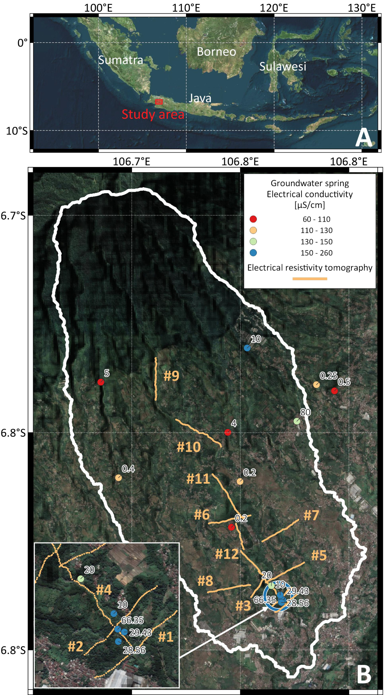
(A) Location map of the study area in Indonesia. (B) Map of the investigated surface watershed (delineated in white) with location of surveyed groundwater springs (solid circles), and of the twelve numbered ERT profiles. The springs are colored as a function of the water electrical conductivity and labeled with spring discharge (in L/s).
In this context, it becomes crucial to understand the distribution of renewable water flows through the different compartments of the watershed. However, such quantification is hampered by the heterogeneity of the subsurface, which is composed of volcanic rocks and/or detrital formations that host spatially variable heterogeneous aquifers [Lachassagne et al. 2014; Selles et al. 2015]. The summit of the volcanoes, characterized by steep slopes above 20° and up to 40°, is usually mainly composed of andesitic lava flows and pyroclastic projections. At the foot of these steep slopes, lava flows transition to alternations of detrital and distal ash fallout layers that form peripheral detrital aprons. Lower down, the aprons become alluvial floodplains, with alternating laharic formations and fine-grained soils, which can prevent the upwelling of underlying groundwater, creating artesian aquifers [Toulier et al. 2022]. This layering of geological formations related to the distribution of volcanic formations spatially disconnects the surface watersheds from underground ones [Charlier et al. 2011; Dumont et al. 2021; Vittecoq et al. 2014]. At the same time, geological discontinuities along slopes may allow the release of groundwater at spatially-restricted emergence points, which may substantially contribute to surface water flows [Vittecoq et al. 2019]. These andesitic hydrosystems are complex due to their lateral and vertical heterogeneity and are poorly or not instrumented.
Hydrogeological models are useful tools to better assess water fluxes between the compartments of the water cycle. The existing modelling strategies cover a large spectrum organized along a two-dimensional continuum according to spatial resolutions and process complexities [Hrachowitz and Clark 2017], from lumped, conceptual models to process-based models describing the system from a microscale perspective. Both approaches were applied in andesitic settings. Lumped or semi-distributed holistic reservoir models were developed to accurately capture water exchanges between the atmosphere, the soil, runoff and the subsurface [Cerbelaud et al. 2022; Charlier et al. 2008; Gómez-Delgado et al. 2011; Mottes et al. 2015]. Generally calibrated on river flows, they simplify the complexity of the aquifers that is induced by the andesitic volcano structure. Process-based models solving Richards’ equation and Darcy’s law have also been developed to represent physical processes [Chang et al. 2020; He et al. 2008; Lo et al. 2021; Satapona et al. 2018]. In this case, the finite element mesh is constructed by incorporating geological and hydrogeological features to simulate the water table with a calibration on monitored boreholes. Nevertheless, the surface/underground exchanges are significantly simplified limiting the representativeness of the aquifers in the watershed water cycle. Both approaches rely heavily on data, either to calibrate model parameters or to prescribe the geometry and hydrodynamic properties of geological and hydrogeological features. To calibrate and/or to validate the models, continuous river discharge or piezometric data are required over long record periods to represent annual and interannual variability. This traditional calibration framework does not allow for the integration of non-continuous data or expert knowledge that could improve the performance of the simulations [Gharari et al. 2014].
To model andesitic hydrosystems, we argue that representing the surface/underground exchanges is mandatory while at the same time keeping the representativeness of the aquifers consistent with the heterogeneity of the environment. In addition, the management of weakly instrumented watersheds would benefit from the development of an iterative approach between field measurements and/or monitoring and modelling approach to incrementally improve water cycle quantification. Such an approach may provide early-stage estimations of water fluxes and highlight which data are missing for more accurate estimation. The development of such water cycle simulation is strongly needed in order to sustainably manage water resources and to quantify the impact of climate on water availability.
To achieve this, our study develops a methodology to structure the progressive characterization of a minimally instrumented hydrosystem. The objective is to obtain a first simulation usable for water use management while guiding future surveys and monitoring. This approach was designed for a previously hydrogeologically unknown mountainous watershed in West Java (Figure 1A). Located on the volcano chain crossing the island, this mountainous area is strategic for a wide variety of water use, such as for population supply, irrigation, and industry. However, these hydrosystems are considered hydrogeologically unknown because their geological structures, extensions and dynamics have not yet been determined, which is necessary to improve their management. The only hydrological data available in the watershed is the discharge of the artesian springs used to supply the local population and/or industrial uses. Consequently, a better understanding of the hydrosystems and their functioning is necessary to define sustainable water management. Our study is divided into three steps: (i) hydrosystem characterization through a multidisciplinary study to set up a conceptual model; (ii) the transformation of the conceptual model into a numerical one; and (iii) the calibration of this latter using field data.
2. Material and method
2.1. Methodological approach
To set up the conceptual model, we need to define the structure, characterize the compartiments of the water cycle and estimate their behaviors to construct a meaningful model. First, the volcanic structure and aquifer(s)/impervious bodie(s) geometries have to be determined. For decades, geophysical methods demonstrated their strength to image volcanic structures and identify aquifer geometries [Descloitres et al. 1997; Dumont et al. 2019; Gresse et al. 2021; Vittecoq et al. 2019]. We thus imaged the hydrogeological structure of the watershed using 2D electrical resistivity tomography (ERT) combined with a geological review of surface outcrops and of artesian borehole lithological data. Second, the different aquifers need to be identified and characterized between shallow, perched, and deep reservoirs [Join et al. 2016]. Geochemistry has proven its efficiency in identifying the recharge areas and the main characteristics of the aquifer [Bénard et al. 2019; Join et al. 2016; Toulier et al. 2019]. To do so, we used geochemical analyses and discharge measurements to identify both perched and deep artesian aquifers. This further allowed defining the extent of each identified aquifer type. In addition, the elevation of aquifer recharge was assessed using water stable isotope of rainfall within the watershed and deep artesian aquifers. Lastly, hydrological monitoring of river or spring discharges are an important data to compute water balance between the different water reservoirs of the watershed [Charlier et al. 2011; Vittecoq et al. 2019]. To overcome the lack of such dataset, a rough surface water balance was obtained from point measurements of river flow, which are used to estimate surface water/groundwater flows.
As the model relies on limited information while integrating the whole water cycle, we used a lumped model. The production function adopts the equations of Thornthwaite [1948], while the model storage discharge equation is derived from Perrin et al. [2003]. We applied a Bayesian approach, the multiple-try differential evolution adaptive Metropolis (MT-DREAMZS) to account for the uncertainty in model parameters calibration [Laloy et al. 2015]. The starting probability distribution of the parameters is set as uniform within a threshold estimated from field measurements. Multiple runs of Markov chains then allow transforming the a priori distribution functions into a posteriori probability distribution functions [de Marsily et al. 1999]. This probabilistic exploration of the model parameters space, framed by field interpretations, allows (i) to improve the representability of the water cycle simulation, and (ii) to guide future field characterization by estimating the influence of each parameter on the simulation uncertainty. Thus future field surveys or instrumentation can be optimized using the simulation guidelines.
2.2. Study area
The study site is located on the southern flanks of the Salak volcano, which culminates at 2900 m a.s.l. (Figure 1). This volcano is part of the mountain belt that stretches along the center of the island of Java from west to east. The study area straddles the surface drainage limit between the northern and southern sides of the island. Water resources of the watershed supply local populations as well as agricultural and industrial activities. While the main agricultural use consists of irrigating rice fields by river diversion, other activities are supplied by spring captation or pumping into wells. It is therefore essential to characterize renewable water volumes between the different components of this hydrosystem to maintain a base flow sufficient to sustain local biodiversity and local communities.
2.3. Field measurements
2.3.1. Geomorphology
The geological description of the Salak volcano is still limited. Therefore, we applied a geomorphological analysis to define its main geological units. In particular, slopes and land roughness allow to distinguish areas underlained by lava flows from those underlained by detrital deposits, as described by Selles et al. [2015]. Surface topography characterization was performed on a digital elevation model (DEM) calculated from the Advanced Land Observing Satellite dataset [ALOS—Tadono et al. 2014]. With a resolution of 5 m, the ALOS DEM provides an accurate depiction of the slopes morphology of Salak volcano. The DEM geodesic reference is EPSG 32748—WGS 84/UTM zone 48S. The DEM was used to extract slope maps and delineate surface watersheds using the QGIS software (v3.10.11—https://www.qgis.org/). A pit-filling algorithm (r.fill.dir from the GRASS v7.8.4 package) was used to remove local depressions and other artifacts. The filled DEM was then used to define the watersheds and the hydrographic network using the “r.watershed” function from the GRASS v7.8.4 package. The slope map was calculated using the slope function of the GDAL v3.1.4 package.
2.3.2. Geophysics
To confirm the geomorphological classification of land surfaces into geological units and to provide some insights on the underlying geology, geophysical and geological campaigns were conducted during two field surveys. The first, conducted in December 2020, focused initially on the immediate surroundings of the artesian springs (Figure 1), before proceeding upstream in order to explore the artesian structure extension. Artesian spring water is collected into shallow boreholes, which logging data provide deep geological information. This initial survey was meant to understand the geological parameters controlling the location of the artesian springs, and to collect the geological information at depth needed to assist geophysical imaging interpretations. A second survey was conducted in June 2021 in order to complete geophysical imaging, such as to obtain a nearly continuous longitudinal geophysical section from the artesian springs area up to the break-in-slope marking the transition from the core of the volcano to the surrounding detrital accumulation zone.
During these two surveys, a total of 12 ERT profiles were acquired using an IRIS Instruments Syscal Pro resistivity meter (http://www.iris-instruments.com/syscal-pro.html). All 2D lines were acquired using 64 electrodes with a 10 m spacing and some roll-along specified in Table 1. Acquisition sequences were defined with Wenner–Schlumberger set up, which provides the best trade-off between shallow resolution and depth of investigation [Dahlin and Zhou 2004]. Each measurement was stacked 3 to 6 times with imposed electrical potential of 800 mV. The measurement time window was 500 ms.
Summary of ERT acquisition parameters, which provides for each of the 12 profiles the total length, number of electrodes and the roll-along. No roll-along was implemented along profiles #8, #11 and #12. However, profile #8 is composed of two profiles with an overlap of 310 m, whereas profiles #11 and #12 do not overlap. The two processing columns present the number of data obtained after (without gap-fillers) and before processing, with indication of the percentage of data retained for the inversion. The last column summarizes the absolute error of the inverted model for each profiles. All the profiles are located in Figure 1
| ERT profile | Length (m) | Electrodes | Roll-along | After processing | Before processing | Absolute error (%) |
|---|---|---|---|---|---|---|
| #1 | 630 | 64 | — | 1100 | 966 (88%) | 6.20 |
| #2 | 630 | 64 | — | 1100 | 1023 (93%) | 10.45 |
| #3 | 630 | 64 | — | 1010 | 821 (81%) | 8.99 |
| #4 | 950 | 64 | 32 | 1944 | 1592 (82%) | 6.68 |
| #5 | 950 | 64 | 32 | 1920 | 1720 (90%) | 8.25 |
| #6 | 950 | 64 | 32 | 1944 | 1716 (88%) | 9.72 |
| #7 | 950 | 64 | 32 | 1944 | 1698 (87%) | 15.09 |
| #8 | 950 | 2 × 64 | — | 2200 | 1700 (77%) | 14.36 |
| #9 | 950 | 64 | 32 | 1920 | 1749 (91%) | 16.75 |
| #10 | 1190 | 64 | 32 + 24 | 2520 | 2434 (97%) | 13.25 |
| #11 | 630 × 2 | 2 × 64 | — | 2110 | 2015 (95%) | 7.96 & 3.15 |
| #12 | 630 × 2 | 2 × 64 | — | 2200 | 1944 (88%) | 4.03 & 4.78 |
After field acquisition, ERT and roll-along data were merged and processed using Prosys III software (v1.05, https://www.iris-instruments.com/fr/download.html#processing). In order to delete gap-fillers measurements, as well as measurements with negative apparent resistivity, low intensity and/or low electrical potential data were filtered out. Finally, data with poor standard deviation (above 10%) and insufficient stacking were also removed.
Data were then inverted using l1 norm in Res2dinv software version 3.59.121. The result is presented after 3 iterations. Similar parameters were used to invert all ERT profiles. The width of model grid cells was set to half the electrode spacing. The thickness of the top layer corresponds to 120% of the cell width, and the layer thickness increases by a factor of 1%. The depth of the model is defined with a vertical extension of 5%. The damping factors used are: (i) 0.15 for the initial, (ii) 0.02 for the minimum, and (iii) 5 for the top layer. The flatness ratio is set at 1 to ensure the imaging of both vertical and horizontal structures. Finally, the depth of investigation is estimated using a sensitivity estimation of the inverted resistivity model [Marescot et al. 2003; Oldenburg and Li 1999]. This approach uses two inversions with different initial models and calculates the difference between the two inverted results. Here, we considered that if that difference exceeds 10%, the inverted resistivity model is not valid. Inversions yielding differences between 5 and 10% are regarded as poorly reliable but still informative.
2D-inverted resistivity profiles were ground-proofed near the artesian springs using available geological logs defined with the drilling cores. They allowed us to identify the geological formations corresponding to the imaged geoelectrical layers. The ERT profiles obtained during the second survey allow us extending these interpretations up the slope, combined with surface geological observations.
2.3.3. Hydrology and geochemistry
The study site is located in Java Island characterized by a tropical climate. The year is divided in two seasons: the wet season characterized by strong moonson rainfall (October–March); the dry season with less or no rainfall at all [April–September; Dumont et al. 2022]. The annual rainfall varies from 2 to 5 m/year, while the daily average temperature ranges from 18 to 25 °C.
Alongside the geophysical surveys, springs were inventoried. Their discharges and physico-chemical properties were measured in the field and water samples were taken for further analyses, in particular laboratory measurements of major elements and isotopic ratios. Major elements analysis has been proceded by UnPad ITB laboratory using an ion chromatography instrument. The water isotopic ratios have been estimated by the BATAN laboratory (National Nuclear Energy Agency of Indonesia) using a liquid-water stable isotope analyzer Los Gatos Research DLT-100. Springs were classified according to discharge, major element composition, and groundwater electrical conductivity [Bénard et al. 2019; Charlier et al. 2011; Join et al. 1997, 2016]. Water stable isotopic ratios were used to define the average elevation of the recharge area using the local meteoric line, which we defined from analysis of weighted rainfall collected within the watershed as described in Toulier et al. [2019]. For the watershed, rainfall was collected at four different elevations during the hydrological cycle 2006–2007, both the amount of rainfall and its mean monthly isotopic composition were measured. To characterize the artesian aquifer recharge, three campaigns of water sampling for water stable isotope analysis were carried out from 2006 to 2007. The variations in water stable isotope ratios over the period allowed us to assess the seasonal variability of the recharge processes and to obtain an estimate of the average elevation of the aquifer recharge. Thus the spread of isotopic results informs on changes in the dynamics of the recharge from dry to wet seasons.
Once the hydrogeological structure of the subsurface was defined, it was necessary to understand the distribution of water flow and its dynamics. This step was hampered by the absence of long-term monitoring of river discharges within the surface watershed. Besides, artesian aquifers extension is generally large and disconnected from the surface drainage network. On the one hand, part of the subsurface flow could not be quantified with hydrological monitoring. On the other hand, the model must represent the functioning of the artesian springs and not the whole system in order to be calibrated on the available spring discharges. The river flow measurements undertaken during the 2019 dry season and the 2020 wet season were used as a constraint for surface discharge evaluation in the model. During these surveys, the discharge was repeatedly measured at downstream locations whereas the upstream rivers were measured only during the wet season. The specific discharge rates (as a function of surface area) derived from these site-specific measurements were used as proxies of the specific runoff of all upstream sectors (central and proximal) in order to compute the total runoff. The difference in flow between the dry and wet seasons provides some preliminary insights on annual variations in the dynamics of the rivers. Nevertheless, this information is not comprehensive enough to be used as input in the models and was therefore only used to constrain the simulation results.
Finally, to constrain the water cycle in the system, we use the discharge of the artesian springs tapped for the drinking water supply of the population (Figure 2). These springs have been gradually instrumented since 2015. It is thus possible to have a partial measurement of the artesian aquifer outlet. Indeed, these measurements do not integrate all the artesian springs identified on the field, nor the underground flows that may not be drained by the springs. Nevertheless, we summed the discharge of all the inventoried springs issuing from the artesian aquifer to obtain one discharge time series of more than 5 years, from 2015 to mid-2021, that recorded the seasonal fluctuations of the system. The climate forcing during this period evolved from one year to another with notably an ENSO (El-Niño Southern Oscillation) event between 2014 and 2016. These data allow us to understand how the system reacts to variable forcings.
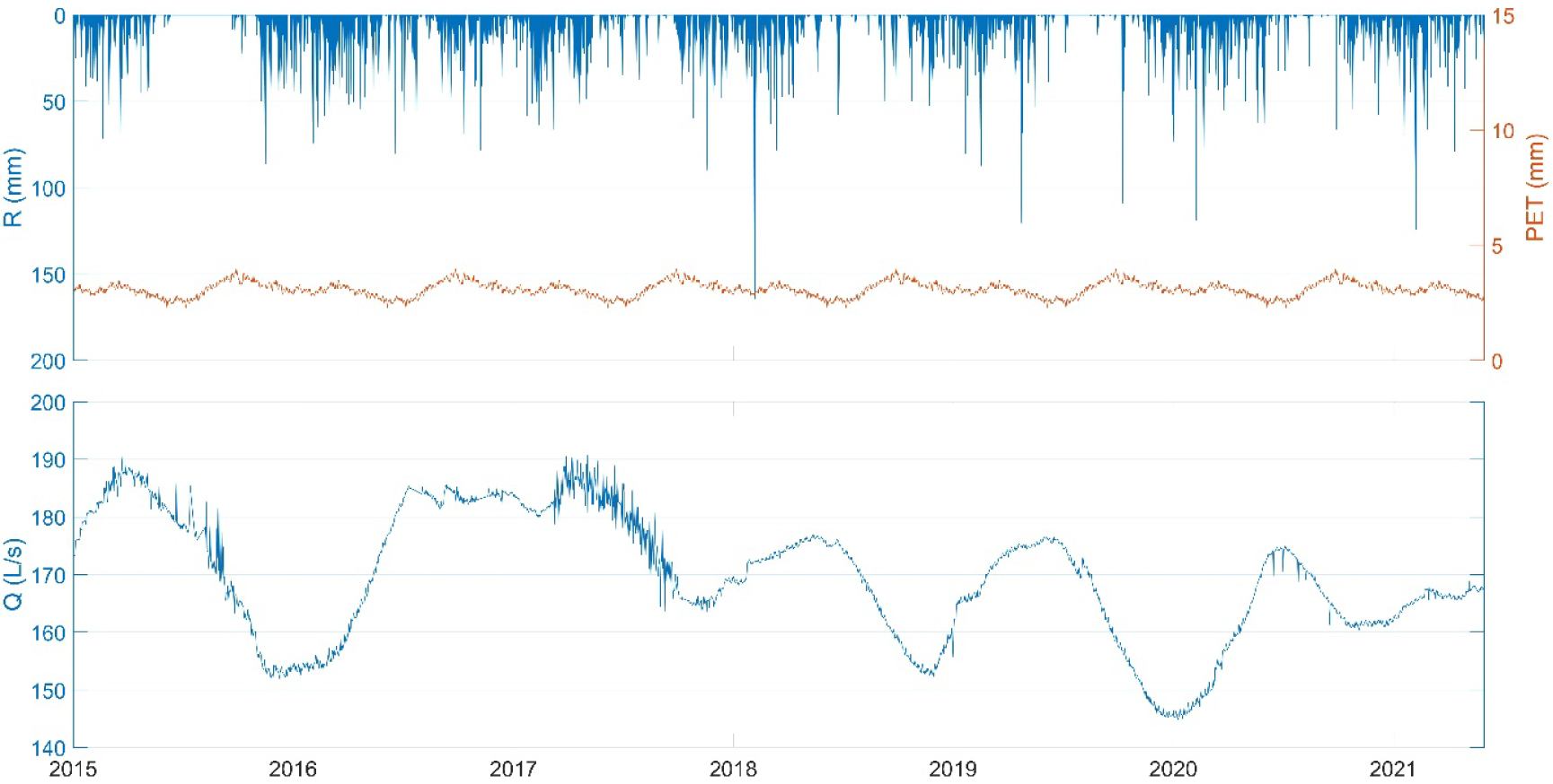
Daily rainfall (R), potential evapotranspiration (PET) and artesian springs discharge (Q) time series from 2015 to mid-2021. Note that the higher noise of the data in 2015 and 2017 is a consequence of the pressure device; the noise is not representative of the real discharge of the spring.
2.4. Water cycle simulation
2.4.1. Lumped model structure
Since the final structure of the hydrological model depends directly on the characterization of the hydrosystems, this section will focus on the description of the equations used. The model was chosen to run at the daily timestep in order to account for the strong rainfall events that occur in such a tropical context.
The production function of the model consists of a soil production storage (SW) defined to estimate the balance between rainfall, evaporation, and vegetation transpiration. The Thornthwaite equation is used to compute the effective rainfall (ER) as:
| (1) |
| (2) |
| (3) |
Weather data used for the water cycle simulation come from the Stamet Citeko station of BMKG network (Badan Meteorologi, Klimatologi, dan Geofisika—http://www.bmkg.go.id) located at 14 km north of the watershed. While the station is not within the watershed, the rainfall analysis of Dumont et al. [2022] demonstrated the representativity and accuracy of this weather station monitored from 2000 to 2021 for the studied area (Figure 2). For the estimation of potential evapotranspiration, the Stamet Citeko station is the only station providing long-term climate data (temperature, radiation, wind, sun exposure time per day and relative air humidity) without long gaps. However, due to punctual gaps in the climate data, they have been averaged over the time series to obtain the climatological potential evapotranspiration for each day of the year (Figure 2). This long-term climatic time series allows us to assign a warm-up period to the model from the beginning of 2000 to the end of 2014, the latter corresponding to the beginning of spring discharge measurements. This warm-up period ensures that the model during the studied period is not impacted by the choices of model initialization.
Below the SR reservoir, the ER feeds runoff (RO) and infiltration. Flux allocation is defined by the Baseflow Index (BFI) parameter, used to calculate the infiltration/effective rainfall ratio. Deeper in the ground, the model structure is not defined at this stage, as it depends on spatially varying hydrogeological characteristics. In the model, each reservoir is characterized by a recharge and by the infiltration or the discharge from a shallower reservoir. Its discharge is calculated as a function of the reservoir state using the GR4J model equations [Perrin et al. 2003]. For a reservoir level R (mm), the outflow QR thus depends on its current filling level R and its maximum capacity Rmax (mm):
| (4) |
2.4.2. Probabilistic parameter exploration
The objective of our methodology is to define the range of possible values for input model parameters, based on the interpretation of field data. This will allow a better linkage between the numerical simulations and field reality while improving the future characterization of the studied hydrosystems. For this reason, the parameterization of the artesian springs flow simulation is based on a probabilistic approach. To do so, we used the multiple-chains differential evolution adaptive Metropolis algorithm [MT-DREAMZS—Laloy et al. 2015] to infer the posterior probability density functions (PDF) of model parameters. At the start, an a priori probability distribution is defined for each parameter. At each iteration, the MT-DREAMZS algorithm uses a latin hypercube sampling to sample parameter values following the statistical methodology presented in Laloy et al. [2015]. Once the parameter values are accepted, the water cycle simulation is run in order to estimate a log-likelihood function used to compare simulation results and measured discharges. The use of multiple Markov chains allows us improving parameter space exploration, limiting the impact of local maximum likelihood on the search for best-fit parameters. In this study, five Markov chains are used with 50,000 iterations per chain. At each iteration, a candidate parameter set is tested via the Metropolis ratio. If it is accepted, the parameter set is validated and integrated into the calibration process.
3. Results and discussion
This section is divided into three parts. First, the conceptual model of the hydrological system is defined using field measurements and observations. Second, this conceptual model is used as the basis to build and set up the numerical lumped model which is used for the probabilistic parameters exploration. Third, the optimal parameter set is used to simulate the spring discharge.
3.1. From observations to a conceptual model
To understand the geological structure of the watershed, our methodology relies on a combination of geological, geomorphological and geophysical information (Figure 3). In addition, hydrogeological knowledge such as the location and properties of the springs are of prime importance to decipher the structure of the conceptual model.
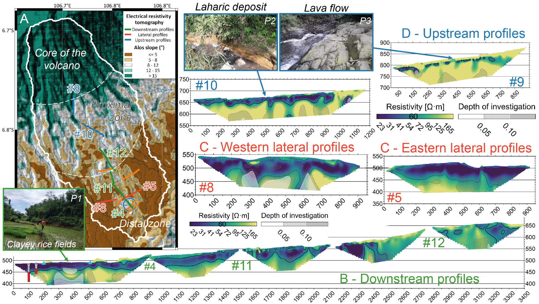
(A) Slopes map of the watershed extracted from the ALOS DEM with the location of the ERT profiles, (B) the downstream profiles starting from the artesian springs area (#4, #11 and #12—green), (C) lateral profiles oriented west–east (#5 and #8—red), and (D) upstream profiles (#9 and #10—blue). The distance along the profiles is presented in m (X axis), as well as the elevation (Y axis). Profiles not presented here are in orange in the map (A). In the slopes map, three geomorphological zones are delineated as: core of the volcano (slope > 15°), proximal (slope from 8° to 15°) and distal (slope < 8°) zones. The three field pictures illustrate the different types of vegetation cover and geological outcrops encountered in the catchment, with clayey rice fields (P1), laharic deposits of the proximal zone (P2), and lava formations of the core of the volcano (P3). In the lowest profile, two artesian wells are located with laharic formations in grey and pyroclastic ones in red. The two nearest springs are located with blue triangles. Masquer
(A) Slopes map of the watershed extracted from the ALOS DEM with the location of the ERT profiles, (B) the downstream profiles starting from the artesian springs area (#4, #11 and #12—green), (C) lateral profiles oriented west–east (#5 and #8—red), and (D) upstream profiles ... Lire la suite
3.1.1. Geomorphological and geophysical results
The slopes map allows dividing the watershed into three zones: the core of the volcano is characterized by steep slopes (average: 23.9°) and, on the opposite, the distal zone by lower slopes (average: 5.5°); the intermediate proximal zone shows variable slopes between 5° and 20° (Figures 3A and 4). In the latter, field geological observations showed that several morphological forms correspond to lava flow fronts, indicating that it is the meeting zone between lava flows tracking from the core of the volcano and the detrital deposits of the distal zone. Downstream of these massive flows, the valley is particularly eroded with slopes of up to 12°, which contrasts with the low erosion of the distal area. The outcrop of lava flow may have disconnected this area from the upper part of the watershed, limiting alluvium deposit or mark the upper limit of regressive erosion coming from downstream. This particular feature allows the underlying formations to outcrop.
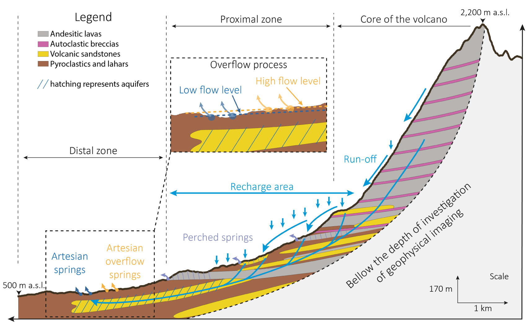
2D conceptual hydrogeological model of the volcano slope. The water flows are represented by blue arrows. A zoom of the artesian springs area provides information on the artesian aquifer water level and the overflow process.
The ERT profiles provide an imagery of the structures at depth (Figure 3B–D). The lowest profile stretches from the artesian springs zone to the lower limit of the proximal zone. These profiles were geologically and hydrogeologically calibrated from the gological data of springs and boreholes located near the springs area (Figure 3B). Thus, these ERT profiles reveal a long, from 10 up to 50 m thick, superficial conductive layer (<60 𝛺⋅m), which extends to about 570 m a.s.l. and thickens over a distance of 2400 m. This conductive layer corresponds to a clayey laharic formation identified in the wells. There it constitutes an aquiclude that seals the underlying resistive (>60 𝛺⋅m) artesian aquifer. The artesian aquifer corresponds in the wells to mildly reworked volcanic breccias, pyroclastic rocks, and sandstones. This main deep reservoir feeds several high discharge (>10 L/s) springs observed in the springs area. Groundwater flows out from the aquifer through the locally thinner (notably in incised valleys) and/or locally more permeable laharic formations (Figure 4). Additional ERT profiles performed immediately downstream the spring area show that the aquifer is bounded there to the south-east by clayey conductive formations; this is an important feature as it surely prevents any groundwater to flow downstream the artesian springs. The western and eastern lateral ERT profiles confirm that both the aquifer and its confining layer extend laterally West and East. The deep resistive aquifer layer is less resistive in the western part, while it deepens towards the eastern limit. Unfortunately, these lateral limits of the aquifer were not reached by the current #5 and 8 ERT profiles (Figure 3C). However, given the absence of other known artesian springs laterally (see Figure 7 below), the aquifer is not expected to extend much farther than the chosen surface watershed boundaries.
At the transition between the distal and the proximal zones, a few tens of meters in elevation above the upper limit of the aquifer confining layer, the ERT profiles reveal a thick resistive layer (80–150 𝛺⋅m) that reaches the surface on a steep slope (8–15°). Both the morphology and outcrops confirm a lava flow front issuing from the North. From this elevation, a conductive layer consistent with laharic outcrops is present in the areas with the shallow slopes (<8°). At the limit with the core of the volcano, the conductive layer deepens and becomes thinner (as seen in #9). This conductive layer is thus comprised between two resistive bodies (Figure 3D). The proximal zone appears as a transition area between a reworked-pyroclastics dominant area (downstream) and a lava-flow dominant area (upstream). There, groundwater may flow from lava-flow to sandstone aquifers. There might also be surface–groundwater interactions, with both springs issuing from aquifers and, locally, streams infiltrating to aquifers. In the core of the volcano, only lava flows and breccias deposits crop out, which is consistent with alternating thinner conductive (lahars) and thicker resistive (lava flows) layers (Figure 3D).
3.1.2. Geochemical and isotopic results
Location and characterization of springs (discharge, geochemical and isotopic analyses) combined with hydrological measurements on streams complete this geological/geomorphological/geophysical analysis. In the distal zone, there are no springs outside the spring zone (blue points in Figure 1). There, artesian springs are characterized by high discharges (between 10 and 40 L/s) and the highest measured electrical conductivities (130 to 150 μS/cm—Figure 5A). During the wet season, additional artesian springs were identified a little further upstream in the field. This highlights that the artesian aquifer discharge varies according to the hydraulic head in the aquifer which is controlled by seasonal recharge. When this latter increases, temporary springs appear at a higher elevation. Several of these springs only flow during the wet season, accommodating fluctuations in discharge of the aquifer throughout the year (Figure 4). Upstream, in the proximal zone, all springs have a lower discharge rate (⩽5 L/s) and lower electrical conductivities (<120 μS/cm—Figure 5A) which suggests the existence of only local perched aquifers of small spatial extent (Figure 4).
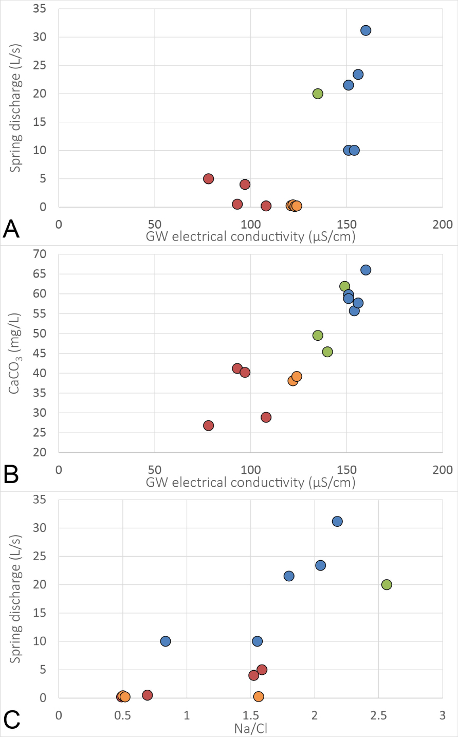
(A) Spring discharge as a function of the groundwater (GW) electrical conductivity; (B) carbonate mass concentration as a function of the groundwater (GW) electrical conductivity; and (C) spring discharge as a function of sodium/chloride ratio (concentrations are transformed in meq/L to estimate this ratio). The dot colors correspond to groundwater electrical conductivity clusters defined in Figure 1. Blue and green dots correspond to artesian springs.
Globally, the groundwater electrical conductivity is well correlated to the discharge of the springs as well as to the carbonate mass concentration, which may be related to the contact time between groundwater and the aquifer rocks (Figure 5A and B). The sodium/chloride (Na/Cl) ratio, defined by Join et al. [1997], tends to be well correlated with flow discharge (Figure 5C). Higher ratios (longer water/rock interactions) are usually reached in the deep artesian aquifer while the shallow aquifers exhibit lower Na/Cl ratios (Na/Cl < 1.6). The Na/Cl ratios support previous insights indicating that the proximal springs are fed by small extention aquifers while the artesian springs are supported by an extensive deep one (Figure 4).
Then, oxygen and hydrogen stable isotope ratios allowed to estimate the elevation of the recharge area of the artesian aquifer (Figure 6). The measurement of monthly weigthed rainfall isotopic ratios allow to estimate the water local meteoric line of Salak volcano (SMWL; 𝛿2H‰ = 7.83 ×𝛿18O + 12.35). This meteoric line is consistent with Toulier et al. [2019] Bromo–Tenger meteoric line (BMWL; 𝛿2H‰ = 7.71 ×𝛿18O + 12.37). As for Toulier et al. [2019], the SMWL appears above the global and local meteoric line, GMWL and LMWL respectively, demonstrating the local topographic effect on rainfall composition. The oxygen and deuterium ratios measured in the artesian aquifer have a low range of variation throughout the sampling periods compared to the variation observed in other springs and rivers sampled in the same time in the watershed (Figure 6A). This stability confirms the important inertia of the artesian aquifer.
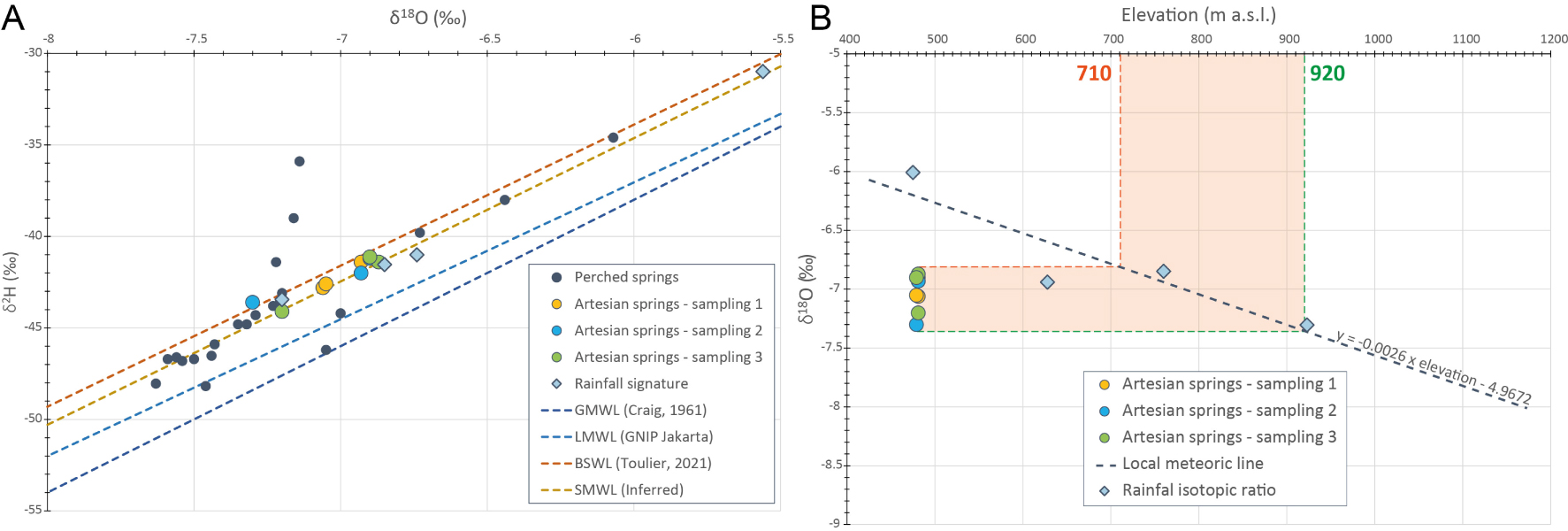
(A) Oxygen and deuterium isotopic ratios of weighted rainfall (in light blue), artesian springs (in yellow, blue and green according to the sampling periods) and other springs and rivers of the watershed (in black). Meteoric lines are plotted with dashed lines: dark blue for the global meteoric water line [Craig 1961]; light blue for the local meteoric line (GNIP station of Jakarta); orange for Bromo line [Toulier et al. 2019]; and the Salak line (inferred in this study). (B) Analysis of water stable isotopes to estimate the mean elevation of the recharge of the artesian aquifer. Masquer
(A) Oxygen and deuterium isotopic ratios of weighted rainfall (in light blue), artesian springs (in yellow, blue and green according to the sampling periods) and other springs and rivers of the watershed (in black). Meteoric lines are plotted with dashed lines: ... Lire la suite
In addition, the monitoring of stable isotopes of rainwater sampled at four different elevations (475, 628, 760 and 923 m) during the 2006–2007 hydrological year was used to calibrate the local elevation meteoric line: 𝛿18O = −0.0026 ×elevation − 4.9672. We can thus estimate that the aquifer recharge occurs within the elevation range between 710 and 920 m a.s.l. according to Figure 6B, indicating a median recharge area of about 800 m a.s.l. Considering that the artesian aquifer recharge area can hardly extend below about 600 m a.s.l. (see section above on the geophysical interpretations; 200 m below the 800 m a.s.l. median recharge area), we can conclude that rainfall precipitated up to about 1000 m a.s.l. may recharge the artesian aquifer (200 m above the 800 m a.s.l. median recharge area), provided effective rainfall does not vary too much within this elevation range [Toulier et al. 2019]. However, as recharge may also result from runoff after rainfall events, the upper limit of the recharge area is probably lower than 1000 m a.s.l. (Figure 4) as runoff may come from higher elevations than the recharge upper limit. More detailed research in that area should be performed to precise this upper limit.
3.1.3. Hydrological results
The final step in the characterization of the hydrosystem is the surface water dynamics. Concerning surface water, river discharge measurements showed limited flows in the upstream sectors with specific flows of 17 to 20 L/s/km2 (river discharges between 120 and 200 L/s for a subcatchment surface of 6.5 to 11 km2). Downstream, the river flow increases up to 4140 L/s for a contributive surface of 40 km2 (specific discharge of 104 L/s/km2). The overall watershed discharge evolves during the year with a decrease of the discharge by a factor of 8 during the dry season (a discharge of 510 L/s and a specific one of 12.75 L/s/km2). In fact, during the dry season, rainfall decreases drastically resulting in the drying up of perched springs and upstream rivers. The map of specific discharges is presented in Supplementary Material A.
The analysis of the artesian springs discharge time series allows a better understanding of the seasonal variations of hydraulic heads in the aquifer. These variations are buffered in the deep aquifer, with low water periods between October and March depending on the year. The annual variations range between 150 and 190 L/s. The suspected overflow effect described previously from the temporary discharge of the springs located above the springs area zone appears to be supported by a flow threshold around 190 L/s.
In this section, the combination of geological observations, geophysical imagery, slope analysis, hydrological and hydrogeological observations as well as geochemical and isotopic analyses allowed to characterize the hydrosystem’s structure and limits, and provided a first robust hydrological conceptual model (Figure 4). The numerical model will then be based on this conceptual model. Nevertheless, the numerical model will also enable challenge and, if possible, confirm the coherence of this conceptual model.
3.1.4. Water cycle characterization summary
In order to assist in understanding the transition from the conceptual to the numerical model, the characteristics of the hydrosystem are summarized below. In the studied area, a thick clayey layer extends over the distal area. It thins out at the center of the distal zone of the watershed, at places where the slope increases locally. At depth, the underlying aquifer is confined below this impervious layer over most of the area. Locally, thanks to the thinnings of this clayey layer, it outflows through several artesian springs (Figure 7). Outside the artesian spring area (blue circle in Figure 7), no significant springs were identified in this distal zone. The layering imaged at low elevation in the distal zone appears to change in the proximal zone farther upslope. One of the reasons is the presence of lava flow fronts in the steep areas of the proximal zone, which could act as local, perched aquifers. These perched aquifers feed springs with different geochemical signatures (Figure 5), characterized by a lower mineralization, and shorter residence time than the deep aquifer, typical of local, perched aquifers [Join et al. 2016]. Detritic and laharic accumulations probably produce the conductive clayey layers imaged near the surface. Farther upstream, slopes are directly underlain by high permeability pyroclastic flows with no interstratified low-permeability detrital formations. There, the increase in slope, and progressive disappearance of clayey deposits blanketing the land surface, agree with the average recharge elevation estimated from stable isotopes (Figure 7). However, this result does not prevent the existence of a recharge from the core volcano slopes and lower proximal zone.
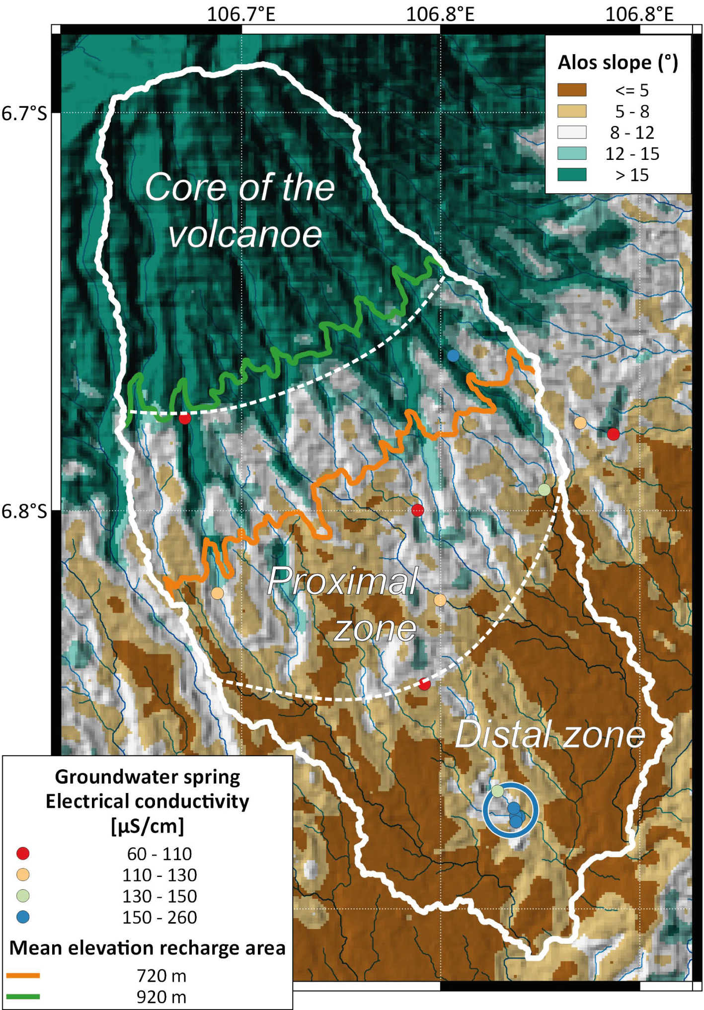
Slopes of the watershed extracted from ALOS DEM with the delimitation of the core of the volcano, proximal and medial zones. The artesian springs located in the artesian spring area (blue circle) are characterized by high electrical conductivity (130–250 μS/cm) and perched springs by a lower electrical conductivity (60–120 μS/cm). The mean recharge area is delimited by the lower (710 m, orange line) and higher (920 m, green line) limits estimated from water stable isotopes.
3.2. Probabilistic lumped model
3.2.1. Lumped model structure
The structure of the hydrological model is then set up based on hydrosystem architecture described in Figure 8. The lumped model relies on the equations previously presented in Section 2.4.
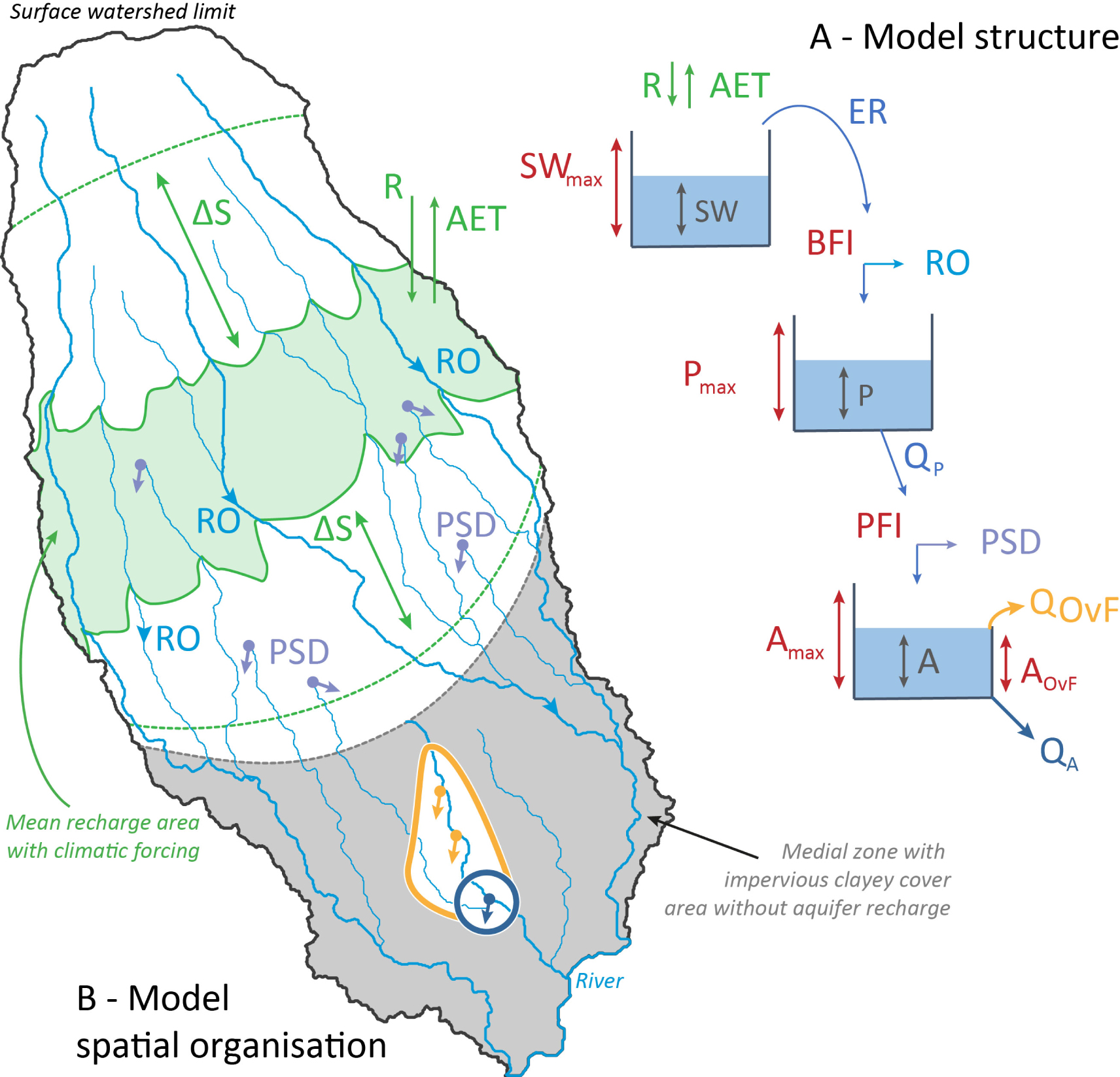
Structure (A) and spatial organization (B) of the lumped model. In the structure, the parameters are represented in red, climatic forcing in green, model fluxes in light blue and model states in dark blue. In the map, the surface of the recharge area (S) of the model is represented in green. This surface may evolve according to the results of the isotopic ratios (±𝛥S). The artesian (blue circle) and the overflow springs areas (yellow extension) are delineated according to the eroded area in the slopes map (Figure 7). Masquer
Structure (A) and spatial organization (B) of the lumped model. In the structure, the parameters are represented in red, climatic forcing in green, model fluxes in light blue and model states in dark blue. In the map, the surface of the recharge ... Lire la suite
At the top of the model, seasonal fluctuations in rainfall (R) and actual evapotranspiration (AET) forcings control the water level in the soil water (SW) reservoir (Equations (1)–(3)—Figure 8). When the SW reservoir is full (>SWmax), excess water is transformed into effective rainfall (ER). The ER is then divided between runoff (RO), which supplies stream water, and infiltration to the shallow perched aquifer reservoir (P). The parting of ER fluxes is defined by the BFI parameter. The discharge of P (QP) is calculated using Equation (4) and divided into perched springs discharge (PSD) and the recharge of the artesian aquifer (A), according to the perched flow index ratio (PFI). This latter corresponds to the ratio between water feeding perched springs discharge, and water reaching the artesian aquifer. The discharge of reservoir A (QA) represents the artesian spring’s outflow, which is simulated and compared to spring discharge measurements during the calibration process (blue circle—Figure 8B). However, considering that some springs only discharge during the wet season, we considered instead that, above a specific water level in reservoir A (threshold AOvF), the discharge of the springs no longer increases. This parameter consists of a filling ratio of reservoir A. This can be explained by the drainage of groundwater towards non-perennial springs (not instrumented) located at slightly higher elevations (yellow extension—Figure 8B). To represent that shortcut in the model, an overflow function (OvF) was implemented into the artesian reservoir A. The excess water is thus transformed into a non-perennial springs discharge (QOvF).
Consequently, the numerical model resulting from the proposed conceptual model is thus composed of three reservoirs: SW, P and A (Figure 8A). Each of them possesses a maximum filling level that constitutes 3 calibrated parameters: SWmax, Pmax, Amax. The other four parameters of the model are indexes BFI and PFI, overflow threshold level AOvF, and the extension of the recharge area S that supplies the artesian springs (Figure 8A). As the discharge series we want to simulate correspond to only a part of the water flows in the watershed, the model extension should include only a part of the watershed. We delineate this feeding catchment S as the area enclosed within the elevation range of the recharge area, inferred from the analysis of the isotopic ratios of the artesian springs (Figure 6B). This surface can evolve towards a higher or lower altitude according to the hydrological cycles and its extension can also change.
3.2.2. Probabilistic exploration of lumped model parameters
The calibration of the model is conducted using the probabilistic approach MT-DREAMZS. For this purpose, uniform a priori probability distributions are defined for each parameter. Field data are used to define the range of parameter values to improve the convergence of the simulations, prevent convergence toward local solutions, and improve the representativeness of spring discharge simulations.
The first parameter SWmax represents the thickness of the soil reservoir that serves as an interface between the atmosphere, the vegetation and the deep reservoirs. In the watershed, soils are thin on lava flows but thicken substantially on detrital formations. The a priori distribution of soil thickness SW was allowed to vary between 50 and 500 mm (of water). The ranges of values of reservoir filling parameters of the perched and deep reservoirs, Pmax and Amax, were set based on geophysical imaging. In the central and proximal zones, resistant horizons, interpreted as perched aquifers, have thicknesses ranging from 1 to 20 m. At depth, the artesian aquifer displays thicknesses ranging from 10 m up to 60 m. The size of the feeding catchment S is about 7.2 km2 from the area enclosed within the elevation of the recharge area, inferred from the analysis of the isotopic ratios. However, the recharge may take place over a larger area as demonstrated by Toulier et al. [2019]. Therefore, the contributing catchment can expand up to 30 km2 according to the surface watershed (Figure 8B). An in-situ observable range of values for the remaining three parameters can not be constrained with field data. We therefore allowed these parameters to vary over a very broad range. Indexes BFI and PFI thus vary from 0 to 1, and overflow AOvF varies between 10 and 50% of the A reservoir thickness.
Once the size of the parameters space was set, 50,000 MT-DREAMZS iterations were run on 5 Markov chains (see Supplementary Material B). Over all these iterations, 1401 sets of parameters were validated by the Metropolis ratio. Each parameter quickly converged to a best-fit value. Parameters appear uncorrelated with each other, highlighting their independence (see the correlation matrix in Supplementary Materials C). Out of the 1401 simulations, the last 25% are considered as a posteriori simulation and are used for the analysis of the results. The posterior PDFs are thus reported on Figure 9.
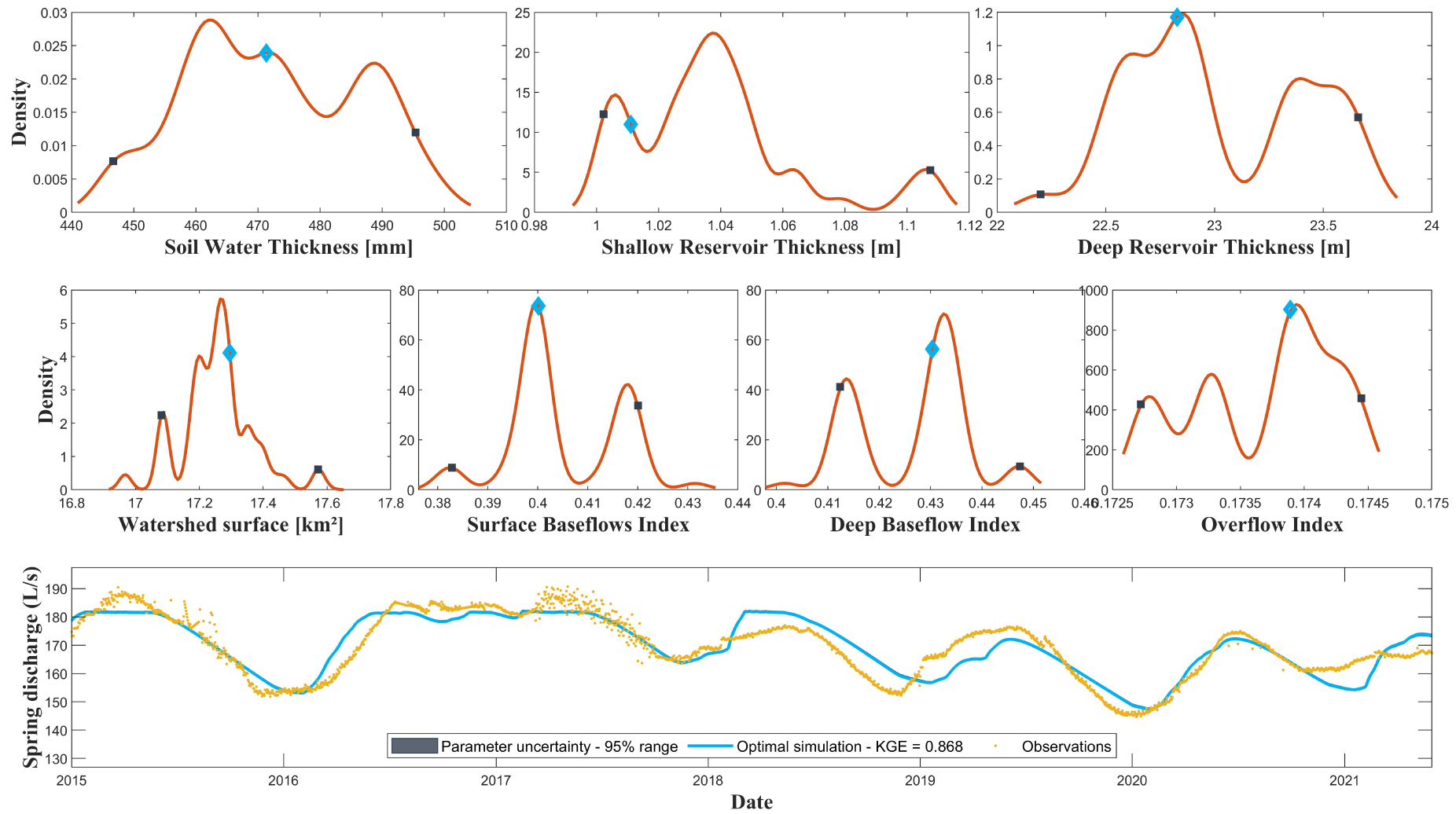
Probabilistic exploration of lumped model parameters. The red lines represent the seven probability density functions (PDFs) of the parameters. In each line, the posterior distribution of each parameter is defined by dark square. The optimum parameter value is pointed with a blue diamond. The bottom part represents the artesian springs observed discharge with yellow dots, the optimum simulated discharge in blue with the 95% range parameters uncertainty. The 95% range parameter uncertainty represents the variability in simulated spring discharge as a function of the posterior distribution of parameters. It does not represent a comprehensive assessment of the model uncertainties. The parameter uncertainty is small since the posterior distribution of the parameters is narrow. Masquer
Probabilistic exploration of lumped model parameters. The red lines represent the seven probability density functions (PDFs) of the parameters. In each line, the posterior distribution of each parameter is defined by dark square. The optimum parameter value is pointed with ... Lire la suite
The parameter exploration converges to a restricted range of posterior distributions. The best-fit values of SWmax, Pmax and Amax are 471 mm, 1.01 and 22.83 m respectively, each one is close to the probability peak (Figure 9—top panel). Their posterior distribution at the 95% confidence level is restricted between 447 and 495 mm, 1 and 1.11 m, and 22.2 and 23.66 m, respectively. These results demonstrate fairly good confidence in the parameters estimates despite the low constraint on the deep reservoir. The area is also fairly well constrained, between 17.1 and 17.6 km2, with an optimum at 17.3 km2. The two indexes, BFI and PFI, are also focused around their optimal values 0.4 and 0.43 respectively (range from 0.38 to 0.42 and 0.41 to 0.44). Finally, the optimum of AOvF is located at 0.174 (range from 0.173 to 0.175). The good convergence of the Bayesian approach is remarkable on the simulated flow curve since the 95% prediction interval is narrow (Figure 9—bottom panel).
With a KGE score of 0.87, the simulation represents fairly well the dynamics of the artesian springs, especially at the beginning (2015–2017) and for the hydrological cycle (2019–2020). In between, the quality of the simulation is slightly altered. For example, in 2018, the simulation overestimates the discharge during the wet season and early 2019, the simulated discharge keeps decreasing while the observations increased. Also, the simulation underestimates the recharge of the aquifer at the end of 2020 and the start of 2021. Although the simulation is less efficient during these periods, the model error does not exceed 6% of the observed discharge.
The last model validation is based on the use of river specific flows measured in the field. To do this, our model allows computing the discharge of the different water flows over the watershed (Figure 10). The simulated watershed runoff (RO) varies between 0 and 7 m3/s on average with larger floods up to 16 m3/s. The perched springs discharge (PSD) varies between 0.2 and 1.5 m3/s. The artesian springs discharge (QA) is completly buffered between 150 and 180 L/s.
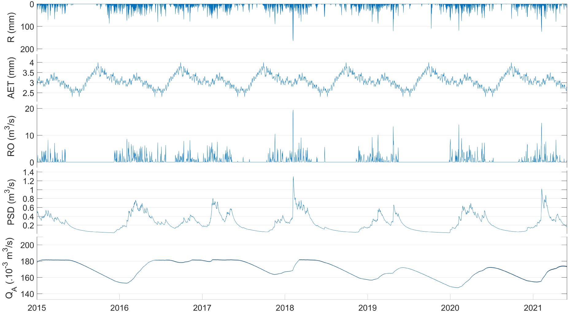
Simulation inputs and outputs simulated at daily basis: rainfall (R), actual evapotranspiration (AET), runoff (RO), perched spring discharge (PSD), and the artesian spring discharge (QA). The climatic forcings are in mm/day while the surface and groundwater flows are in m3/s.
From these simulations, we extracted the average values corresponding to the months of field measurements. In December 2020, the runoff measured in the field was 18 to 20 L/s/km2. In comparison, the median specific flow of the model during December is 13 L/s/km2. However, the simulated floods occurring during this period have a strong impact on the average specific flow (50 L/s/km2). Considering the dry/wet period comparison, while in the field the river flow is 8 times higher during the wet season, the model simulates an increase of a factor of 5.5. Nevertheless, the high-frequency variability of the river flow simulated during the wet season is directly related to rainfall dynamics. This high variability complicates the analysis of punctual river measurements. It seems therefore impossible to constrain the model without continuous monitoring of river flows. Herein lies the most important margin of progress to improve the simulations. The implementation of continuous monitoring of river flow, even limited in time, will improve the robustness of the simulations. This monitoring should be made at the outlet of the surface watershed as well as upstream in the proximal zone to calibrate perched and the artesian aquifer water balance. To do so, the upstream river should be instrumented to calibrate BFI parameter, as well as the downstream one for PFI.
3.2.3. Interest of probabilist approach for andesitic hydrosystem simulation
In this study, we developed a hydrological model aiming to represent the water cycle on the flanks of an andesitic volcano. To do so, we followed a two-step framework including (i) the proposal of a model structure as simple as possible to represent the complex and heterogenous surface- and ground-water behaviors; (ii) a probabilistic approach aiming at determining model parameters using a wider diversity of punctual measurements data.
Regarding the first issue, we focused on lumped reservoir models to balance the number of parameters with available data. The flexible structure of such models can be easily adapted to the complex hydrogeological characteristics of the environment [Dubois et al. 2020; Mazzilli et al. 2019]. Such a modelling approach was already implemented in a French West Indies watershed by Charlier et al. [2008] who set up a conceptual hydrogeological model considering both surface and groundwater flows. Our study goes further by integrating multidisciplinary analyses combining geophysical, geochemical, and isotopic measurements to further constrain the model structure. Both studies show the ability of parsimonious reservoir models to represent complex subsurface flows of minimally instrumented watersheds. In these conditions, we assume that this parsimonious approach of lumped parameters models is the most consistent approach to represent the complexity of the volcanic environment. Process-based models would provide a finer representation of physical processes but would require extensive additional data to set up and validate. Given the amount of available data and the large heterogeneities of the studied areas, the feasibility of such a modelling approach is still to be proven.
Regarding the second aspect, we developed a probabilistic approach aiming at integrating punctual measurements data from a wide variety of disciplines. Prior distributions of parameter values were derived using geophysical imagery, geochemical and isotopic analyses as well as expert knowledge, which allows strengthening the confidence in model simulations. In the future, other datasets could be integrated to improve the calibration/validation process as piezometric data [Charlier et al. 2008], geophysical monitoring [Lesparre et al. 2020], or groundwater dating [Kolbe et al. 2016]. The integration of a wider diversity of dataset in water simulation increase the confidence in the processes captured by the model while limiting equifinality issues during the calibration of the model parameters.
Finally, the probabilistic approach provides posterior distribution of parameter values and an estimation of parameter uncertainty instead of a unique set of parameters. This allows representing fairly the parametric uncertainties of the model that are inherently large in poorly gauged environments. However, these parametric results have to be carefully interpreted as (i) DREAM algorithm try to disentangle error source but Bayes’ law suffers from the interaction between individual sources of error (input, output, parameter, and model structure error); and (ii) the DREAM algorithm tends to provide a tighter posterior distribution of parameters than other informal Bayesian approach [Vrugt et al. 2009]. Besides, the analysis of posterior distribution is a first step towards the identification of ways to improve the model structure and parametrization by further field mesurement.
4. Conclusion
The objective of this work was to integrate the multidisciplinary characterization of a previously unknown watershed to build a representative hydrological model of the water cycle in an andesitic volcanic aquifer. This characterization was needed for a better management of the wide variety of water uses for human needs within the watershed, while supporting biodiversity. Unfortunately, this characterization was hampered by a significant lack of measurements. To overcome this difficulty, we defined a parsimonious and realistic conceptual model in order to understand the hydrological behavior in function of the climate forcing.
The multidisciplinary field characterization provides a characterization of hydrosystem structure as well as the identification of the aquifers distributed over the watershed. Our study revealed an extensive artesian aquifer at the foot of the andesite volcano confined by detritic clayey deposits. When the thickness of this latter decreases, due to erosion and/or thinner deposits, the aquifer supports significant artesian springs (150–190 L/s). On the slopes of the volcano, the alternation of lava flows and detritic formations allows the development of perched aquifers with small extension. While the recharge of both types of aquifers occurs on the volcano slopes, extension and outlet location of the aquifers induce spatially different behaviors. This characterization based on data analysis and field observations allowed to set up a conceptual lumped model characterized by various reservoirs representing closely the different functions observed. This model is used to simulate the artesian springs discharge.
Due to data scarcity, we improved the hydrological simulation by implementing a probabilistic estimation of the model parameters. The field characterization allowed to define a uniform a priori distribution for some of the parameters. From these distributions, the use of several Markov chains allowed to test a wide range of parameter sets while limiting the influence of local optima. The Bayesian simulation allows providing a PDF to analyze the uncertainty of parameter values. Finally, the uncertainty could be represented on the simulated water flows to estimate its impact.
This combination of a field-based approach and the probabilistic integration of field measurements allows reinforcing the simulation of ungauged watersheds. Despite a limited constraint on surface river flow, this simulation allows today to better manage the groundwater resource in this strategic sector. In the future, new field acquisitions could be guided by the simulation results. To go further, it would be possible to integrate into the model other reservoirs to represent the main anthropogenic activities that develop rapidly in the watershed. First, an exchange function with urban areas could be added. This function would withdraw groundwater from the deep aquifer and discharge water to the surface. A second reservoir representing the rice terraces would allow the model to be refined by integrating the delayed effect of surface flows, the increase in evaporation, and the influence on the recharge of agricultural practices.
Conflicts of interest
Authors have no conflict of interest to declare.
Acknowledgements
This project has been carried out within the collaboration between Sorbonne University (METIS laboratory), Water Institute by Evian, Danone Aqua group and the Universitas Padjajaran (UNPAD). This research was funded by Sorbonne University and Danone Aqua, in the framework of Danone Aqua Waterstewardship acceleration plan on watershed preservation. The authors are grateful to Damien Jougnot (Sorbonne University—METIS laboratory) for his help in the implementation of the MT-DREAMZS algorithm.
Vous devez vous connecter pour continuer.
S'authentifier