Can marine protected areas enhance both economic and biological situations?

Dominique Ami; Pierre Cartigny; Alain Rapaport

doi:10.1016/j.crvi.2004.10.018

Biological modelling / Biomodélisation

Can marine protected areas enhance both economic and biological situations?
[Des réserves maritimes peuvent-elles être bénéfiques à la fois sur les plans économique et biologique ?]

Présenté par : Pierre Auger

Dominique Ami ¹ ; Pierre Cartigny ¹ ; Alain Rapaport ²

¹ GREQAM, 2, rue de la Charité, 13002 Marseille, France
² UMR « Analyse des systèmes et biométrie », 2, place Viala, 34060 Montpellier, France

Comptes Rendus. Biologies, Volume 328 (2005) no. 4, pp. 357-366.

Résumés

Anglais
Français

This paper investigates impacts of the creation of Marine Protected Areas (MPAs), in both economic and biological perspectives. The economic indicator is defined as the sum of discounted benefits derived from exploitation of the resource in the fishery sector, assumed to be optimally managed. The biological indicator is taken as the stock density of the resource. The basic fishery model (C.W. Clark, Mathematical Bioeconomics: The Optimal Management of Renewable Resources, second ed., John Wiley and Sons, New York, 1990) will serve as a convenient benchmark in comparing results with those that are derived from a model of two patchy populations (cf. R. Hannesson, Marine reserves: what would they accomplish, Mar. Resour. Econ. 13 (1998) 159). In the latter, a crucial characteristic is the migration coefficient with describes biological linkages between protected and unprotected areas. A set of situations where both economic and biological criteria are enhanced, after introducing a MPA, is presented. These results are obtained with the help of numerical simulations.

Cet article étudie les impacts de la création de zones de réserves maritimes dans des perspectives aussi bien biologiques qu'économiques. L'indicateur économique est défini comme la somme actualisée des revenus de l'exploitation de la resource, dans un secteur de pêche supposé géré de façon optimale. L'indicateur biologique est la densité du stock de la resource. Le modèle classique de Clark (Mathematical Bioecomics: The Optimal Management of Renewable Resources, second ed., John Wiley and Sons, New York, 1990) sert de « benchmark » dans la comparaison des résultats avec ceux dérivés d'un modèle d'une population répartie en deux zones (cf. R. Hannesson, Marine reserves: what would thet accomplish, Mar. Resour. Econ. 13 (1998) 159). Dans ce dernier, une hypothèse cruciale repose sur le coefficient de migration qui décrit les échanges biologiques entre la zone protégée et celle qui ne l'est pas. Un ensemble de situations où les critères économique et biologique sont favorisés, après l'installation d'une réserve, est proposé. Ces résultats sont obtenus à l'aide de simulations numériques.

Métadonnées

Reçu le : 2004-03-02
Accepté le : 2004-10-20
Publié le : 2005-02-05

PMID

DOI : 10.1016/j.crvi.2004.10.018

Keywords: Fisheries economics, Marine reserves, Calculus of variations
Mot clés : Economie des pêches, Réserves marines, Calcul des variations

Affiliations des auteurs :

Dominique Ami ¹ ; Pierre Cartigny ¹ ; Alain Rapaport ²

¹ GREQAM, 2, rue de la Charité, 13002 Marseille, France
² UMR « Analyse des systèmes et biométrie », 2, place Viala, 34060 Montpellier, France

@article{CRBIOL_2005__328_4_357_0,
     author = {Dominique Ami and Pierre Cartigny and Alain Rapaport},
     title = {Can marine protected areas enhance both economic and biological situations?},
     journal = {Comptes Rendus. Biologies},
     pages = {357--366},
     publisher = {Elsevier},
     volume = {328},
     number = {4},
     year = {2005},
     doi = {10.1016/j.crvi.2004.10.018},
     language = {en},
}

TY  - JOUR
AU  - Dominique Ami
AU  - Pierre Cartigny
AU  - Alain Rapaport
TI  - Can marine protected areas enhance both economic and biological situations?
JO  - Comptes Rendus. Biologies
PY  - 2005
SP  - 357
EP  - 366
VL  - 328
IS  - 4
PB  - Elsevier
DO  - 10.1016/j.crvi.2004.10.018
LA  - en
ID  - CRBIOL_2005__328_4_357_0
ER  -

%0 Journal Article
%A Dominique Ami
%A Pierre Cartigny
%A Alain Rapaport
%T Can marine protected areas enhance both economic and biological situations?
%J Comptes Rendus. Biologies
%D 2005
%P 357-366
%V 328
%N 4
%I Elsevier
%R 10.1016/j.crvi.2004.10.018
%G en
%F CRBIOL_2005__328_4_357_0

Dominique Ami; Pierre Cartigny; Alain Rapaport. Can marine protected areas enhance both economic and biological situations?. Comptes Rendus. Biologies, Volume 328 (2005) no. 4, pp. 357-366. doi : 10.1016/j.crvi.2004.10.018. https://comptes-rendus.academie-sciences.fr/biologies/articles/10.1016/j.crvi.2004.10.018/

Version originale du texte intégral

1 Introduction

Recently one could observe an upsurge of contributions concerning impacts of Marine Protected Areas (MPAs). This growing interest for MPAs can be explained first by the various benefits expected from the creation of MPAs. These benefits can be broadly classified under three kinds: ecosystem preservation, fisheries management and development of the nonextractive recreational activities (Boncoeur et al. [2]). Secondly, MPAs are often presented as a new tool to control over-exploitation of the marine resource, which is a serious worldwide problem. Third, another motivation is that many MPAs have already been practiced all over the world. Lauck et al. [10] assert that MPAs can be envisaged as a kind of insurance against scientific uncertainty or stocks assessments or effectiveness of regulation errors.

Similar to Arnason [1], our paper is concerned with the study of theoretical conditions under which MPAs may be also economically beneficial. In biological perspective, MPAs generally increase abundance and average size of exploited species within their boundaries. There is an evidence that benefits may be exported to surrounding regions in some cases. We have restricted our attention to impacts on the fishing sector under the assumption that fishery is optimally managed by fishery managers (whether individuals or committees). In such a perfect world, we show that creation of a well designed MPA can improve biological situations within MPA boundaries, as well as economic benefits from the fishing activity outside its boundaries.

Following Hannesson [7], we use here a model where a given fishing ground is split into two sub-areas. One of them is set aside as a MPA. It is assumed that fish stock within the boundaries of MPA and stock fish into the surrounding area are linked by migration patterns of the resource. This framework is a variant of the spatial model developed by Sanchirico and Wilen [13]. This setting appears to be powerful and leaves open many possibilities with regard to what kind of migration may take place between stocks. It might be used for modeling a wide-ranging scale of problems. For instance, discussing the existence and the stability of an optimal harvesting policy (Dubey et al. [6]), or determining the optimal size of a MPA in the stochastic case (Conrad [5]).

Obviously, existence of economic benefits from the fishing activity outside MPA boundaries is contingent on the nature of biological linkages between areas. It will be assumed here that biological linkages are mainly dependent on adequate design of the MPA. By design we mean essentially here location and size. These are characteristics of major importance to appraise a migration coefficient that gives us some information on the fish mobility (cf. Houde [9]). In the present paper, it is then assumed that the knowledge of the migration coefficient allows one to identify and then choose the locations that have the highest potential for the implementation of a MPA. Therefore, the migration coefficient can be considered as a decision variable of fishery managers.

More precisely, the basic harvesting model, as it can be found, for instance, in Clark [4], is used as a benchmark. Though our study appears also as an optimal harvesting problem, we work, as Clark did, in the calculus of variation framework. Indeed the interior solutions of the optimal control problem, the only ones we are interested in, are straightforwardly obtained in this setting.

A MPA consideration is added to the basic model, leading to a model of two patchy populations that allows us to explore the possible effects of MPA. The biological and economics impacts, both within and beyond the borders of the MPA, are highlighted.

Optimal steady states, expressed in terms of fishing effort and stock density, are determined in both the basic and the patchy models. For the latter one, the optimal migration coefficient, i.e., the value where potential effect of MPA implementation should be highest, is obtained. Optimal benefits, with or without MPA, are compared. Conditions under which a MPA creation will theoretically enhance both biological (i.e. the stock density) and economic (i.e., the present value of the exploitation) situations are obtained. Unfortunately, it is likely uneasy to reach in practice the optimal value of the migration coefficient. Some simulations are therefore used to explore the sensitivity of our results with respect to the migration coefficient. It is shown numerically that the domain of the parameter for which the presence of a MPA is theoretically beneficial is reasonably large.

The paper is organized as follows. In Section 2 the basic fishery model is presented. In Section 3 the MPA component is added to the model. The implications for economics benefits and for the biomass are then explored. In Section 4 a set of results of simulations is shown. The last section summarizes the major conclusions and suggest some additional lines of research, for which is should be taken into account additional arguments in favor of MPA implementations.

2 The basic fishery model

Consider a fish stock distributed over a given area that we represent by its density X (defined as the ratio of the stock over the carrying capacity of the area). In accordance with classical modeling, the growth of the biomass density is given by:

\dot{X} = F (X) - h (t) = F (X) - q E (t) X (t)

(1)

where

F (\cdot)

is the natural density growth function and

h (t)

the capture rate.

E (t)

is the fishing effort at time t and q stands for the catchability coefficient. The density growth function

F (\cdot)

is defined from

[0, 1]

R^{+}

. It is assumed to be regular, strictly concave and such that

F (0) = F (1) = 0

The standard economic theory claims that fishery managers maximise the profits from harvesting, which amounts to deal with the following optimization problem $(P)$ :

\max_{E (\cdot)} \int_{t = 0}^{+ \infty} e^{- δ t} (P q X (t) - c) E (t) d t s.t.: \dot{X} = F (X) - q E (t) X, X (0) = X_{0}

(2)

0 ⩽ E (t) ⩽ E_{\max}, 0 ⩽ X (t) ⩽ 1

(3)

where P is the value (or price) of the carrying capacity and c is the cost per unit of effort, both assumed to be constant.

δ > 0

is the instantaneous discount rate.

According to (2), for all trajectories s.t. $X (t) \neq 0$ for any $t ⩾ 0$ , we obtain a calculus of variations problem over an infinite horizon (4), equivalent to $(P)$ :

\max_{X (\cdot)} \int_{t = 0}^{+ \infty} e^{- δ t} (P - \frac{c}{q X (t)}) (F (X (t)) - \dot{X} (t)) d t

(4)

where

X (\cdot)

belongs to some space of paths (piecewise continuously differentiable functions s.t. the improper integral converges and constraints (2), (3) are satisfied). If an interior solution exists, it must satisfy the classical Euler necessary condition, which takes here the following expression.

(\frac{P q X (t)}{c} - 1) (δ - F^{'} (X (t))) - \frac{F (X (t))}{X (t)} = 0

(5)

It is well known that in this “singular case”, i.e., when (5) determines an unique stationary path

X^{*}

, the optimal solutions are the most-rapid approach paths to

X^{*}

[4,8].

2.1 Optimality conditions

For the study of the solutions of (5), we introduce a function $R (\cdot)$ , that will be also useful in the next sections:

R (X) : = (\frac{P q}{c} X - 1) (δ - F^{'} (X)) - \frac{F (X)}{X}

(6)

If there exists a solution $X^{*} \in] 0, 1]$ of $R (X) = 0$ , then we observe that the corresponding fishing effort $E^{*} = \frac{F (X^{*})}{q X^{*}}$ , satisfies the constraint (3) for a large enough bound $E_{\max}$ . Moreover when the density growth function obeys the logistic law (i.e. $F (X) = r X (1 - X)$ ), the existence of a unique singular solution for the problem $(P)$ is proved as soon as $P q > c$ (cf. Appendix B).

2.2 Optimal fishing effort and fishery profit

When an optimal stationary solution $X^{*}$ exists, the associated optimal fishing effort $E^{*}$ satisfies

E^{*} = (δ - F^{'} (X^{*})) \frac{(P q X^{*} - c)}{c q}

(7)

with the profit

J^{*} = \frac{(P q X^{*} - c) E^{*}}{δ}

P q X^{*} ⩾ c

E^{*}

is feasible (i.e. nonnegative, because

F^{'} (X^{*}) < δ

, see the expression (6)), and the fishery profit is nonnegative.

If $P q X^{*} < c$ , $E^{*}$ is negative. The profit associated to any feasible value of stationary E is nonpositive. The optimal solution consists in no fishing.

3 Marine protected areas and optimality

Let us consider that we have an optimally managed fishery and examine the impacts of the introduction of a MPA in such a situation. We claim that under an efficient fisheries management system, a MPA, properly defined and implemented, may enhance both economic benefits and fish stocks.

The model used here is structurally very similar to Hannesson's model [7]. It deals with sub-populations distributed in two patches interacting through migration. This is a variant of the spatial model developed by Sanchirico and Wilen [12].

It is assumed that the migration depends only on the biomass densities in each area (i.e., the ratio of stock over carrying capacity). The simplest migration model is based on diffusion, which depends merely upon the difference between the respective densities of patches. Therefore migration occurs if a disparity arises between the respective biomass densities inside and outside the MPA.

Following Conrad [5], Hannesson [7], it is presumed that the carrying capacity is increasing with the patch size. Nevertheless, we assume here that the carrying capacity of the MPA is always very small compared to the overall carrying capacity, which is equivalent to claim that the carrying capacity of the unprotected area is (almost) not modified by the existence of a MPA. Consequently, we consider here that the value P of the carrying capacity in the harvesting area is not modified by the creation of a MPA.

Suppose also that this spatial consideration allows us to distinguish the population behavior between two dynamics, as follows. The growth of the sub-population density into the MPA is governed by the dynamics:

{\dot{X}}_{1} = F_{1} (X_{1}) + λ (X_{2} - X_{1})

(8)

while the growth of the sub-population density into the fishing area is governed by the dynamics:

{\dot{X}}_{2} = F_{2} (X_{2}) - λ (X_{2} - X_{1}) - q E_{2} X_{2}

(9)

We assume that the growth functions

F_{i} (\cdot)

(

i = 1, 2

) fulfill the same assumptions than

F (\cdot)

in the basic model.

First, we examine existence and stability of equilibria of the coupled dynamics $(8, 9)$ , when λ and $E_{2}$ are given positive numbers. This dynamical system admits at most one equilibrium $(X_{1}^{e}, X_{2}^{e})$ different from $(0, 0)$ , which is necessarily asymptotically stable (see Proposition 1 in Appendix A). Moreover, in the logistic case, we can derive a necessary and sufficient condition for the existence of such an equilibrium (see Corollary 2 in Appendix A).

Secondly, let us pay attention to the migration coefficient λ. There are many possibilities with regard to what kind of migration may take place between stocks inside and outside a MPA. The relationship we shall focus on here could allow mutual in- and out-migration. For $λ > 0$ , this is the classical migration by diffusion: the flow is oriented from the highest density towards the lowest.

Particular cases when $λ < 0$ can be interpreted as “sink-source” systems in which flows from patch to patch are constrained by biological effects, like stream that can reverse the migration due to differential of densities. We shall explain further why we get interested only in cases for which $λ > 0$ . It is clear that the possible values of this parameter are also strongly related to biological and spatial parameters, such as the fish mobility and the size of the protected area. Real estimation of these values would require deeper biological and experimental studies on concrete cases. Such studies would also certainly reveal in which extent a decision maker can really influence the value of this parameter, for instance, choosing the size and the location of the protected area. However, one can consider that fishery managers can decide which patch can be close and when. Thus, it can be considered that fishery managers can decide, in some extent, of the value of λ, and possibly change it with time. Nevertheless, our objective in this theoretical work is mainly to show that there exists a set of values for this parameter, for which a protected area is beneficial for both the biological and economical view points. The mathematical technique we use for finding such “good” values is to consider first the parameter λ as if it was a real control variable, i.e. a function of time $λ (\cdot)$ . Then, the optimal steady state solution of the associated problem gives us the “best” stationary value $λ^{*}$ for this parameter. The simulations we have launched for different values about this optimal one show that the beneficial situation is quite robust for a reasonably large set of values of λ.

In this setting, one has to deal with the following optimal control problem $(P_{MPA})$ with the two controls $E_{2} (\cdot)$ and $λ (\cdot)$ . The objective is to maximize the present value of the fishery obtained from the exploitation of the resource, that takes place only in the unprotected area.

\max_{E_{2} (\cdot), λ (\cdot)} \int_{t = 0}^{+ \infty} e^{- δ t} (P q X_{2} (t) - c) E_{2} (t) d t

s.t.: {\dot{X}}_{1} = F_{1} (X_{1}) + λ (t) (X_{2} - X_{1}) {\dot{X}}_{2} = F_{2} (X_{2}) - λ (t) (X_{2} - X_{1}) - q E_{2} (t) X_{2} 0 ⩽ E_{2} (t) ⩽ E_{\max}, 0 ⩽ X_{i} (t) ⩽ 1 (i = 1, 2) X_{1} (0), X_{2} (0) given

For the time being no positivity constraint on the control variable

λ (\cdot)

is stated. As before, for all trajectories s.t.

X_{2} (t) \neq 0

for any

t ⩾ 0

, the problem

(P_{MPA})

is equivalent to a calculus of variations problem:

\max_{X_{1} (\cdot), X_{2} (\cdot)} \int_{t = 0}^{+ \infty} e^{- δ t} (P - \frac{c}{q X_{2} (t)}) [F_{1} (X_{1} (t)) + F_{2} (X_{2} (t)) - {\dot{X}}_{1} (t) - {\dot{X}}_{2} (t)] d t

(10)

3.1 Optimality conditions

The Euler first order optimality condition gives the following equations:

{\dot{X}}_{1} = X_{2} (\frac{P q}{c} X_{2} - 1) (F_{2}^{'} (X_{2}) - δ) + F_{1} (X_{1}) + F_{2} (X_{2})

{\dot{X}}_{2} = X_{2} (\frac{P q}{c} X_{2} - 1) (δ - F_{1}^{'} (X_{1}))

We first study candidate optimal steady state solutions $(X_{1}^{*}, X_{2}^{*})$ . If $F_{1} (X_{1}^{*}) \neq 0$ , then the following equations are satisfied.

δ - F_{1}^{'} (X_{1}^{*}) = 0

(11)

X_{2}^{*} (\frac{P q}{c} X_{2}^{*} - 1) (F_{2}^{'} (X_{2}^{*}) - δ) + F_{1} (X_{1}^{*}) + F_{2} (X_{2}^{*}) = 0

(12)

Given the regularity assumptions on

F_{1}

, for any

δ \in] 0, F_{1}^{'} (0)]

, there exists at least one solution

X_{1}^{*}

of (11). We notice also that the expression

X_{2}^{*} (\frac{P q}{c} X_{2}^{*} - 1) (F_{2}^{'} (X_{2}^{*}) - δ)

is necessarily non-null. Therefore, Eq. (12) can be re-written as

R (X_{2}^{*}) = H (X_{2}^{*}) : = \frac{F_{1} (X_{1}^{*})}{X_{2}^{*}}

where

R (\cdot)

has been defined in (6). Thus

X_{2}^{*}

can be graphically interpreted as the intersection of the graphs of the two functions

R (\cdot)

and

H (\cdot)

(cf. Fig. 3). In the logistic case, for any

δ \in] 0, r_{1} [

, there exists a unique solution

(X_{1}^{*}, X_{2}^{*})

(cf. Appendix B).

Remark

Up to now, there has been no reason to claim that one of the $X_{i}^{*}$ was necessarily greater than the other. Nevertheless we observe in (8) that optimal steady state solutions with $λ^{*} > 0$ correspond exactly to cases such that $X_{1}^{*} > X_{2}^{*}$ . These are the situations of interest, where the protected area acts as a natural hatchery, as underlying by fishery scientists [3]. Therefore, we shall impose in the following that feasible paths fulfill $λ (\cdot) > 0$ . In the particular case of the logistic growth model, the condition $λ^{*} > 0$ is equivalent to the following one (cf. Appendix B).

R (X_{1}^{*}) > \frac{F_{1} (X_{1}^{*})}{X_{1}^{*}}

(13)

3.2 Optimal fishing effort and fishery benefit

At optimal steady state, the optimal fishing effort can be derived, combining (8), (9) and (12):

E_{2}^{*} = (δ - F_{2}^{'} (X_{2}^{*})) \frac{(P q X_{2}^{*} - c)}{c q}

(14)

while the associated profit is

J_{MPA}^{*} = \frac{1}{q δ c} {(q P X_{2}^{*} - c)}^{2} (δ - F_{2}^{'} (X_{2}^{*}))

(15)

With the same argumentation than in Section 2.2, the optimal solution is feasible (i.e.

E_{2}^{*} ⩾ 0

) exactly when

P q X_{2}^{*} ⩾ c

, and the profit

J_{MPA}^{*}

is then necessarily nonnegative. One deduce also that

δ - F^{'} (X_{2}) > 0

. Recalling (11), one has

δ = F_{1}^{'} (X_{1}^{*})

and consequently

X_{2}^{*}

fulfills the property

F_{1}^{'} (X_{1}^{*}) > F_{2}^{'} (X_{2}^{*})

When

P q X_{2}^{*} < c

, no harvesting is the best solution.

4 Comparison between the two situations

Our goal here is to establish conditions under which a MPA could enhance both economic and the biological situations. We have turned to numerical computation because it seems quite difficult to obtain a complete analytical comparison. In the sequel we shall consider the case where growth functions $F_{i} (\cdot)$ obey the logistic law:

F_{i} (X_{i}) = r_{i} X_{i} (1 - X_{i}) (i = 1, 2)

For simplicity, we introduce the dimensionless price

\tilde{P} = P q / c

We present here some of our numerical results that seem to be particularly relevant for our purpose. For this, we have fixed $r_{2} = 0.2$ and $δ = 0.2$ and let $r_{1} = α r_{2}$ for different values of $α > 1$ . Expressions (6) and (11) become

R (X_{2}) = 0.4 \tilde{P} {(X_{2})}^{2} - 0.2 X_{2} - 0.2

X_{1}^{*} = (α - 1) / (2 α)

The condition (13) guaranteeing that the optimal steady states are feasible (i.e., such that

λ^{*} > 0

) provides the following minimal value for the parameter

\tilde{P}

{\tilde{P}}_{\min} = \frac{α (α^{2} + 4 α - 1)}{{(α - 1)}^{2}}

4.1 Sensitivity analysis with respect to α and $\tilde{P}$

For different values of α and $\tilde{P}$ , we have computed and compared the optimal solutions $(X^{*}, E^{*})$ without MPA and $(X_{1}^{*}, X_{2}^{*}, E_{2}^{*})$ with an optimal MPA. For instance, taking $α = 2$ , we have found $X_{1}^{*} ≃ 0.250$ and ${\tilde{P}}_{\min} ≃ 22$ . The results obtained for different values of the parameter $\tilde{P} > {\tilde{P}}_{\min}$ are presented in Table 1.

$\tilde{P}$	$X^{*}$	$q E^{*}$	$q E^{} X^{}$	$X_{2}^{*}$	$q E_{2}^{*}$	$q E_{2}^{} X_{2}^{}$	$λ^{*}$
24	0.155	0.169	0.0262	0.241	0.462	0.111	8.6
30	0.137	0.172	0.0236	0.221	0.496	0.110	2.6
36	0.125	0.175	0.0219	0.205	0.524	0.107	1.7
42	0.115	0.177	0.0204	0.193	0.550	0.106	1.3
48	0.107	0.178	0.0190	0.183	0.572	0.105	1.1

As expected, we notice that managing a protected area with a higher growth rate (i.e. $r_{1} > r_{2}$ ) can allow higher captures at optimal steady states: $q E_{2}^{*} X_{2}^{*} > q E^{*} X^{*}$ .

4.2 Sensitivity analysis with respect to λ

In practice, it might be difficult to control with accuracy the fish migration between the two areas, and to impose the precise optimal value $λ^{*}$ . So, we study (numerically) the sensitivity of the equilibrium $(X_{1}^{e}, X_{2}^{e})$ of the system (8), (9) with respect to variations of the coefficient λ about the best value $λ^{*}$ , while the harvesting effort $E_{2}$ is set to its optimal value $E_{2}^{*}$ (computed and reported in Table 1).

The equilibrium $(X_{1}^{e}, X_{2}^{e})$ is computed (numerically) as the (unique) solution of a system of equations ${g_{2} (g_{1} (X_{1})) = X_{1}, X_{2} = g_{1} (X_{1})}$ , where the functions $g_{i} (\cdot)$ are made explicit in Appendix A (cf. (A.2)). For instance, for $α = 2$ , we found:

	λ	7	8.6 (optimal)	10
$\tilde{P} = 24$	$X_{1}^{e}$	0.253	0.250	0.249
	$X_{2}^{e}$	0.245	0.241	0.240
	λ	1	1.1 (optimal)	2
$\tilde{P} = 48$	$X_{1}^{e}$	0.272	0.250	0.169
	$X_{2}^{e}$	0.193	0.183	0.139

We notice that the effects of a variation of the migration coefficient on the steady states densities is not very significant. Consequently, the gain in managing a protected area with a migration coefficient about $λ^{*}$ is quite robust.

4.3 Improvement of the fishery value

Now we compare the present value of the fishery with and without a protected area. More precisely, we consider optimal stationary situations, when the decision to create a reserve or to close the existing one is taken. Therefore the present value of the fishery has to take into account the transit period when the biomass densities have to reach the new steady state. We assume that fishery managers have means to prevent migration outside the MPA when this one has been created (this amounts at taking $λ = 0$ in our model). We compare then three possible scenarios.

Scenario 1

There is no protected area and the value of the stock density is at its optimal value $X^{*}$ . Harvesting optimally consists in remaining at the steady state $X^{*}$ with the harvesting effort $E^{*}$ . The associated profit is $J^{*} = \frac{c}{δ} (\tilde{P} X^{*} - 1) E^{*}$ .

Scenario 2

There is no protected area and the value of the stock density is at its optimal value $X^{*}$ . The decision to create an “optimal” protected area has been taken at time 0. So, one has $X_{1} (0) = X_{2} (0) = X^{*}$ . We consider then the harvesting strategy that drives the densities $(X_{1}, X_{2})$ as fast as possible to the optimal values $(X_{1}^{*}, X_{2}^{*})$ , as explicited below.

Consider first the durations $T_{i}$ ( $i = 1, 2$ ) defined as the times for the solutions of the differential equations ${\dot{X}}_{i} = r_{i} X_{i} (1 - X_{i})$ to reach $X_{i}^{*}$ from $X^{*}$ :

T_{i} = \frac{1}{r_{i}} \log (\frac{X_{i}^{*} (1 - X^{*})}{X^{*} (1 - X_{i}^{*})})

Then, two cases are possible, depending on the values of

T_{1}

and

T_{2}

When $T_{1} ⩾ T_{2}$ , the strategy is the following.

(i) Create a protected area at date 0 and prevent fish migration outside the area.
(ii) Stop the harvest at date $T_{1} - T_{2}$ .

When

T_{1} ⩽ T_{2}

, the strategy is the following.

(i) Stop the harvest at date 0.
(ii) Create a protected area at date $r_{1} (T_{2} - T_{1}) / (r_{1} - r_{2})$ and prevent fish migration outside the area.

In both cases, the system reaches

(X_{1}^{*}, X_{2}^{*})

exactly at time

T = \max (T_{1}, T_{2})

. Then, allowing fish migration with a coefficient

λ^{*}

and harvesting at a level

E_{2}^{*}

leave the system at this steady state. The present value at date T of the benefits is

J_{MRAP}^{*} = \frac{c}{δ} (\tilde{P} X_{2}^{*} - 1) E_{2}^{*}

. Then, the present value of the benefits at the date of harvest closure is, in both case:

J_{open} = e^{- δ T_{2}} J_{MRAP}^{*}

Scenario 3

The protected area has been created with a migration coefficient $λ^{*}$ and the stock densities are at their optimal values $X_{1}^{*}$ , $X_{2}^{*}$ . A decision to close the protected area amounts to manage the harvested stock $X_{2}$ as an independent one. Then, the optimal solution is known to reach as fast a possible the value $X^{*} < X_{2}^{*}$ for the stock density, keeping maximal harvesting effort $E_{\max}$ (cf. [4]), and then to stay at the steady state $X^{*}$ with an harvesting effort $E^{*}$ . The associated present value of the fishery is

J_{close} = \int_{t = 0}^{T} e^{- δ t} c (\tilde{P} {\tilde{X}}_{2} (t) - 1) E_{\max} d t + e^{- δ T} J^{*}

where

{\tilde{X}}_{2} (\cdot)

is solution of

{\dot{\tilde{X}}}_{2} = r_{2} {\tilde{X}}_{2} (1 - {\tilde{X}}_{2}) - q E_{\max} {\tilde{X}}_{2}, {\tilde{X}}_{2} (0) = X_{2}^{*}

which can be easily integrated. T is the first time such that

{\tilde{X}}_{2} (T) = X^{*}

, that can be determined analytically.

T = \frac{\log (X_{2}^{*} (q E_{\max} - r_{2} + r_{2} X^{*}))}{q E_{\max} - r_{2}} - \frac{\log (X^{*} (q E_{\max} - r_{2} + r_{2} X_{2}^{*}))}{q E_{\max} - r_{2}}

Notice that the maximum harvesting effort

E_{\max}

needs to be larger than

r_{2} / q

to ensure that the equilibrium

X^{*}

is reachable. For the simulation, we have chosen

E_{\max} = 1 / q

. For instance, for

α = 2

, we obtain:

$\tilde{P}$	$J^{*} (c / q)$	$J_{MRAP}^{*} (c / q)$	$J_{open} (c / q)$	$J_{close} (c / q)$
24	2.3	11	6.4	3.9
30	2.7	14	7.8	4.7
36	3.1	17	9.4	5.4
42	3.4	20	11	6.1
48	3.7	22	12	6.8

We check that, in any case, managing a protected area at the steady state $(X_{1}^{*}, X_{2}^{*})$ with $(E_{2}^{*}, λ^{*})$ improves the present value of the fishery.

5 Conclusion

In this work, impacts of MPA creation have been investigated, on both economic and biological perspectives. Our attention has been focused on the obtention of theoretical conditions leading to economic benefits on the sole fishing sector. More precisely, it has been assumed that the fishery sector is optimally managed by fishery managers (whether individuals or committees). Their optimal behavior consists then in maximizing the present value of the fishery, defined as the sum of the discounted net revenues derived from the exploitation of the resource. With the help of a two patches model, we have found that MPAs should be installed so that the amount of spillover is maximized. Of course, scientific guides are required to advice fishery managers about the design, location and concrete implementation of MPAs.

In further works, it would be useful to examine conditions under which our results are robust under other management rules. Open access regime should be analyzed first. In the open access case, MPA may act as a management tool amongst other complementary management tools.

Secondly, it is well known that there exist other potential benefits that can be advocated in favor of MPA implementation. It should be actually taken into account of consumer or scientific benefits relative to MPA creation. Considering them together with the fishery profits should allow to define a social value of MPAs. The objective of fishery managers should be then to maximize this social value. In the case where the amount of the resource spillover is not sufficient, MPA may lead to loss for the fishery sector. If managers concerns are the only fishery sector benefits, MPA implementation must be given up. If the objective of fishery managers takes into account others potential benefits, the social value of a MPA may still be positive. This work was obviously beyond the purpose of this paper, and would require to assess both economic and social implications of MPAs. Benefits and costs to extractive users (fishermen) but also benefits and costs to nonextractive users, as well as management benefits and costs should be estimated. (Sanchirico et al. [11]). Moreover social value assessment of the MPA would require to take into account equity issues, which may arise because MPAs affect generally different users groups in a disproportionate way.

Appendix A

We study the equilibria of the coupled dynamics

(A.1)

where λ,

E_{2}

are constant positive numbers.

Proposition 1

When the functions $F_{i} (\cdot)$ $(i = 1, 2)$ fulfill the following properties:

(P1) $F_{i} (0) = F_{i} (1) = 0$ ,
(P2) $F_{i} (\cdot)$ is strictly concave,

then the system(A.1)admits at most one equilibrium

(X_{1}^{e}, X_{2}^{e})

different from

(0, 0)

, which is necessarily asymptotically stable.

Proof

Consider the two functions on $[0, 1]$

(A.2)

Then any equilibrium point

(X_{1}^{e}, X_{2}^{e})

of (A.1) is such that

g_{1} (X_{1}^{e}) = X_{2}^{e}

and

g_{2} (X_{2}^{e}) = X_{1}^{e}

. It belongs to the intersection of the graph of the function

g_{1}

and the symmetric of the graph of the function

g_{2}

with respect to the first diagonal.

From the properties (P1) and (P2), we deduce that these functions fulfill the following properties: $g_{i} (0) = 0$ ( $i = 1, 2$ ), $g_{1} (1) = 1$ , $g_{2} (1) = 1 + q E_{2} / λ$ and $g_{i}$ are (strictly) convex ( $i = 1, 2$ ). Moreover we observe also the following properties.

(P3) the graph of $g_{1}$ is below the line segment $(0, 0) – (1, 1)$ (see Fig. 1).
(P4) the symmetric of the graph of $g_{2}$ w.r.t. the first diagonal is above the line segment $(0, 0) – (1 + q E_{2} / λ, 1)$ (see Fig. 1).

Let

(X_{1}^{e}, X_{2}^{e})

and

(X_{1}^{e^{'}}, X_{2}^{e^{'}})

be two non-null equilibria. They both belong to the graph of the function

X_{1} \mapsto g_{1} (X_{1})

, so necessarily

X_{1}^{e} \neq X_{1}^{e^{'}}

. We can assume, without any loss of generality, that

X_{1}^{e^{'}} > X_{1}^{e}

. Consider the line segment

L : (0, 0) – (X_{1}^{e^{'}}, X_{2}^{e^{'}})

. By convexity of

g_{1}

and

g_{2}

, we have the following geometric properties:

– the graph of $g_{1}$ is below $L$ ,
– the symmetric of the graph of $g_{2}$ is above $L$ .

Then

(X_{1}^{e}, X_{2}^{e})

, which belongs also to the intersection of the graph of

g_{1}

and the symmetric of the graph of

g_{2}

, is at the same time below and above

L

, thus a contradiction. So, we deduce that there exists at most one equilibrium different than

(0, 0)

. From the properties (P3)–(P4), we also deduce that any equilibrium point belongs to the domain

D : = {(X_{1}, X_{2}) \in (0, 1]^{2} | \frac{X_{1}}{1 + q E_{2} / λ} ⩽ X_{2} ⩽ X_{1}}

The convexity of

g_{1}

g_{2}

also implies the property:

X_{i} \neq 0 \Rightarrow g_{i} (X_{i}) - X_{i} g_{i}^{'} (X_{i}) < g_{i} (0) = 0

(derivative exists a.e. from the concavity assumption) from which we deduce:

X_{i} > 0, g_{i} (X_{i}) > 0 \Rightarrow g_{i}^{'} (X_{i}) > 0

Then,

g_{2}

is invertible at points

X_{2}

such that

(g_{2} (X_{2}), X_{2}) \in D

. By the inverse function theorem, we have

{(g_{2}^{−1})}^{'} = {(g_{2}^{'})}^{−1}

and the restriction of

g_{2}^{−1}

on the subset

{X_{1} | X_{1} = g_{2} (X_{2}) with (X_{1}, X_{2}) \in D}

is a (strictly) concave function. Finally,

X_{1}^{e}

is a zero of the convex function

h_{1} : X_{1} \mapsto g_{1} (X_{1}) - g_{2}^{−1} (X_{1})

Fig. 1
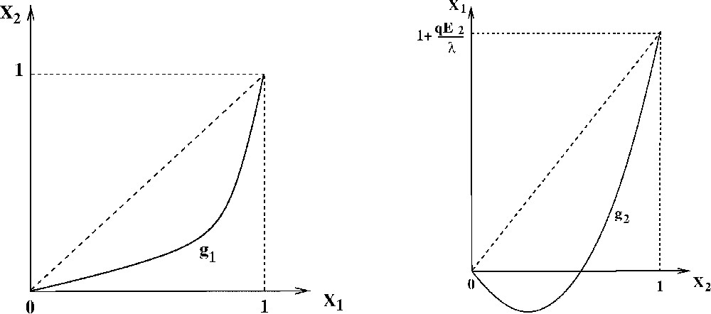
Graphs of the functions $g_{1}$ and $g_{2}$ .

Notice that $h_{1} (0) = 0$ . So $X_{1}^{e}$ , if it exists, must satisfy $h_{1}^{'} (X_{1}^{e}) > 0$ , which amounts to require

g_{1}^{'} (X_{1}^{e}) > {(g_{2}^{−1})}^{'} (X_{1}^{e}) = 1 / g_{2}^{'} (X_{2}^{e})

Thus, we have the necessary conditions

(A.3)

The dynamics (A.1) can be re-written as follows

(A.4)

Finally, conditions (A.3) imply that the Jacobian matrix

J

of the system (A.4) at

(X_{1}^{e}, X_{2}^{e})

fulfills the following properties.

tr (J) = - λ (g_{1}^{'} (X_{1}^{e}) + g_{2}^{'} (X_{2}^{e})) < 0

\det (J) = λ^{2} (g_{1}^{'} (X_{1}^{e}) g_{2}^{'} (X_{2}^{e}) - 1) > 0

from which we deduce the asymptotic stability of the dynamics (A.1) about

(X_{1}^{e}, X_{2}^{e})

. □

Corollary 2

When $F_{i} (X_{i}) = r_{i} X_{i} (1 - X_{i})$ there exists a unique equilibrium $(X_{1}^{e}, X_{2}^{e})$ in $(0, 1]^{2}$ if and only if $q E_{2} < (λ (r_{1} + r_{2}) - r_{1} r_{2}) / (λ - r_{1})$ .

Proof

We have $h_{1} (0) = 0$ and $h_{1} (1) = g_{1} (1) - g_{2}^{−1} (1) = 1 - g_{2}^{−1} (1) > 0$ so there exist $X_{1}^{e} \in (0, 1)$ such that $h_{1} (X_{1}^{e}) = 0$ if and only if $h_{1}^{'} (0) < 0$ , which amounts to require $g_{1}^{'} (0) < {(g_{2}^{−1})}^{'} (0)$ or equivalently $q E_{2} < (λ (r_{1} + r_{2}) - r_{1} r_{2}) / (λ - r_{1})$ . (See Fig. 2.) □

Fig. 2
Existence and uniqueness of $(X_{1}^{e}, X_{2}^{e})$ .

Appendix B

When $F (\cdot)$ is the logistic law, the function $R (\cdot)$ defined in (6) is a convex second order polynomial function. As $R (0) = - δ < 0$ , the convexity provides the existence of a unique $X^{*} > 0$ such that $R (X^{*}) = 0$ . When $P q > c$ , one has $R (1) > 0$ which then ensures that $X^{*}$ belongs to $[0, 1]$ .

Furthermore, by the mean value theorem, there exists an unique $X_{2}^{*} > X^{*}$ such that $R (X_{2}^{*}) = H (X_{2}^{*})$ . To ensure that $X_{2}^{*}$ is feasible (i.e. $X_{2}^{*} < X_{1}^{*}$ ) a necessary condition is to have $R (X_{1}^{*}) > H (X_{1}^{*})$ (cf. Fig. 3).

Bibliographie

[1] R. Arnason Marine reserves: is there an economic justification?, Fish. Center Res. Rep., Volume 9 (2001) no. 8, pp. 19-31

[2] J. Boncoeur; F. Alban; O. Guyader; O. Thebaud Fish, fishers, seals and tourists: economic consequences of creating a marine reserve in a multi-species, multi-activity context, Nat. Resour. Model., Volume 15 (2002) no. 4, pp. 1-25

[3] M.H. Carr; D.C. Reed Conceptual issues relevant to marine harvest refuges: examples from temperate reef fishes, Can. J. Fish. Aquat. Sci., Volume 50 (1993), pp. 2019-2028

[4] C.W. Clark Mathematical Bioeconomics: The Optimal Management of Renewable Resources, John Wiley and Sons, New York, 1990

[5] J.M. Conrad The bioeconomics of marine sanctuaries, J. Bioecon., Volume 1 (1999), pp. 205-217

[6] B. Dubey; P. Chandra; P. Sinha A model for fishery resource with reserve area, Nonlinear Analysis: Real World Appl., Volume 4 (2003), pp. 625-637

[7] R. Hannesson Marine reserves: what would they accomplish, Mar. Resour. Econ., Volume 13 (1998), pp. 159-170

[8] R.F. Hartl; G. Feichtinger A new sufficient condition for most rapid approach paths, J. Optimization Theory Appl., Volume 54 (1987) no. 2, pp. 403-411

[9] E.D. Houde, Testimony on Use of Marine Protected Areas (MPAs) as a Fisheries Management Tool, as a Means to Protect and Restore Marine Ecosystem, and as a Research Tool, Subcommittee on Fisheries Conservation, Wildlife and Oceans, 2002

[10] T. Lauck; C.W. Clark; M. Mangel; G.R. Munro Implementing the precautionary principles in fisheries management through marine reserves, Ecol. Appl., Volume 8 (1998) no. 1, pp. 72-78

[11] J.A. Sanchirico, K.A. Cochran, P.M. Emerson, Marine Protected Areas: Economic and Social Implications, Discussion Paper 02-26, Resource for the Future, 2002

[12] J.A. Sanchirico; J.E. Wilen Bioeconomics of spacial exploitation in a patchy environment, J. Environ. Econ. Manage., Volume 37 (1999), pp. 129-151

[13] J.A. Sanchirico; J.E. Wilen A bioeconomic model of marine reserve creation, J. Environ. Econ. Manage., Volume 42 (2001), pp. 257-276

Commentaires - Politique

Ces articles pourraient vous intéresser

Knowledge and power in integrated coastal management. For a political anthropology of the sea combined with the sciences of the marine environment

Camille Mazé; Tarik Dahou; Olivier Ragueneau; ...

C. R. Géos (2017)

Combined harvesting of a stage structured prey–predator model incorporating cannibalism in competitive environment

Kunal Chakraborty; Kunal Das; Tapan Kumar Kar

C. R. Biol (2013)

The stabilizability of a controlled system describing the dynamics of a fishery

Rachid Mchich; Pierre Auger; Nadia Raïssi

C. R. Biol (2005)

1 Introduction

2 The basic fishery model

2.1 Optimality conditions

2.2 Optimal fishing effort and fishery profit

3 Marine protected areas and optimality

3.1 Optimality conditions

Remark

3.2 Optimal fishing effort and fishery benefit

4 Comparison between the two situations

4.1 Sensitivity analysis with respect to α and P˜

4.2 Sensitivity analysis with respect to λ

4.3 Improvement of the fishery value

Scenario 1

Scenario 2

Scenario 3

5 Conclusion

Appendix A

Proposition 1

Proof

Corollary 2

Proof

Appendix B

4.1 Sensitivity analysis with respect to α and $\tilde{P}$