The stabilizability of a controlled system describing the dynamics of a fishery

Rachid Mchich; Pierre Auger; Nadia Raïssi

doi:10.1016/j.crvi.2004.08.009

Biological modelling / Biomodélisation

The stabilizability of a controlled system describing the dynamics of a fishery
[« Stabilisabilité » d'un système contrôle décrivant la dynamique d'une pêcherie]

Présenté par : Pierre Auger

Rachid Mchich ¹ ; Pierre Auger ¹ ; Nadia Raïssi ²

¹ Laboratoire de biométrie, université Claude-Bernard–Lyon-1, 43, bd du 11-Novembre-1918, 69622 Villeurbanne cedex, France
² Laboratoire SIANO, Département de mathématiques et d'informatique, faculté des sciences, Université Ibn Tofaïl, BP 133, 14000 Kénitra, Morocco

Comptes Rendus. Biologies, Volume 328 (2005) no. 4, pp. 337-350.

Résumés

Anglais
Français

This work presents two stock-effort dynamical models describing the evolution of a fish population growing and moving between two fishing zones, on which it is harvested by a fishing fleet, distributed on the two zones. The first model corresponds to the case of constant displacement rates of the fishing effort, and the second one to fish stock-dependent displacement rates. In equations of the fishing efforts, a control function is introduced as the proportion of the revenue to be invested, for each fleet. The stabilizability analysis of the aggregated model, in the neighborhood of the equilibrium point, enables the determination of a Lyapunov function, which ensures the existence of a stabilizing discontinuous feedback for this model. This enables us to control the system and to lead, in an uniform way, any solution of this system towards this desired equilibrium point.

Ce travail présente deux modèles dynamiques stock-effort décrivant l'évolution d'une population de poissons croissant et se déplaçant entre deux zones de pêche, sur lesquelles elle est exploitée par une flotte de pêche distribuée sur les deux zones. Le premier modèle correspond au cas de taux de déplacement de l'effort de pêche constants, tandis que le second modèle correspond au cas de taux stock-dépendants. Dans les équations des efforts de pêche, une fonction contrôle est introduite, en tant que proportion du revenu investie dans la dynamique de pêche, pour chaque flotte. L'étude de la « stabilisabilité » du modèle agrégé, au voisinage du point d'équilibre, permet la détermination d'une fonction de Lyapunov qui assure l'existence d'un feedback discontinu stabilisant pour ce modèle. Ceci nous permet de contrôler le système et de mener, d'une manière uniforme, n'importe quelle solution de ce système vers le point d'équilibre désiré.

Métadonnées

Reçu le : 2004-03-01
Accepté le : 2004-08-10
Publié le : 2005-02-12

PMID

DOI : 10.1016/j.crvi.2004.08.009

Keywords: Dynamical system, Fishing efforts, Biomass, Investment, Aggregation of variables, Control, Equilibrium points, Feedback, Lyapunov function, Stabilizability
Mot clés : Système dynamique, Efforts de pêche, Biomasse, Investissement, Agrégation des variables, Contrôle, Points d'équilibre, Feedback, Fonction de Lyapunov, Stabilisabilité

Affiliations des auteurs :

Rachid Mchich ¹ ; Pierre Auger ¹ ; Nadia Raïssi ²

@article{CRBIOL_2005__328_4_337_0,
     author = {Rachid Mchich and Pierre Auger and Nadia Ra{\"\i}ssi},
     title = {The stabilizability of a controlled system describing the dynamics of a fishery},
     journal = {Comptes Rendus. Biologies},
     pages = {337--350},
     publisher = {Elsevier},
     volume = {328},
     number = {4},
     year = {2005},
     doi = {10.1016/j.crvi.2004.08.009},
     language = {en},
}

TY  - JOUR
AU  - Rachid Mchich
AU  - Pierre Auger
AU  - Nadia Raïssi
TI  - The stabilizability of a controlled system describing the dynamics of a fishery
JO  - Comptes Rendus. Biologies
PY  - 2005
SP  - 337
EP  - 350
VL  - 328
IS  - 4
PB  - Elsevier
DO  - 10.1016/j.crvi.2004.08.009
LA  - en
ID  - CRBIOL_2005__328_4_337_0
ER  -

%0 Journal Article
%A Rachid Mchich
%A Pierre Auger
%A Nadia Raïssi
%T The stabilizability of a controlled system describing the dynamics of a fishery
%J Comptes Rendus. Biologies
%D 2005
%P 337-350
%V 328
%N 4
%I Elsevier
%R 10.1016/j.crvi.2004.08.009
%G en
%F CRBIOL_2005__328_4_337_0

Rachid Mchich; Pierre Auger; Nadia Raïssi. The stabilizability of a controlled system describing the dynamics of a fishery. Comptes Rendus. Biologies, Volume 328 (2005) no. 4, pp. 337-350. doi : 10.1016/j.crvi.2004.08.009. https://comptes-rendus.academie-sciences.fr/biologies/articles/10.1016/j.crvi.2004.08.009/

Version originale du texte intégral

1 Introduction

The basic subdivision of fishing zones of a coastal state consists on the artisan fishery which operates on 3 miles from the coast, the coastal fishery between 3 and 12 miles and the high sea fishery beyond 12 miles (see [8,20,21]). The adjacent coastal state who is the owner of the resource evolving in his Exclusive Economical Zone, is responsible for the management of the global fishery which is shared by the above mentioned different types of fisheries. So, in order to control the situation, it is important to have a good knowledge of the global evolution of the resource and of the activity related to its exploitation. The fishery management authorities must deal with the possible fishery conflicts resulting, for instance, from the simultaneous exploitation of two fishing zones (we quote, for example, the case of the North American Pacific Salmon [11,13]). Theoretically, each kind of fleet operates in its zone according to its own fishery characteristics. In practice, the fish stock does not remain in a given area and frequently moves between two adjacent zones. Consequently, the fishing vessels do not hesitate to cross the fuzzy boundary between two adjacent zones in order to increase their catch.

In Mchich et al. [9], we built a management bioeconomical model of a fishery, exploited on two fishing zones by two fleets of different characteristics, with constant fishing efforts displacement rates. The model analysis leads to the determination of conditions for the durability of the fishing activity. Then, in Mchich et al. [10], we generalized this work [9] to a model with stock-dependent fishing efforts displacement rates. The analysis of this second model showed the possibility of a limit cycle.

From the point of view of a sustainable fishery, it is better to avoid important variations of the total fish stock and fishing effort, because large periods of time with small stocks and small fishing efforts is not of any social or economic interest. Moreover, if the total stock density becomes too small for some period, then environmental fluctuations could lead to the extinction of the stock. This critical situation has been avoided by introducing a control parameter, in the catchability terms of the model. This made possible to lead the system to a stable equilibrium.

However, it is more realistic to introduce a control function depending on time, rather than a control parameter. This is the aim of this work, where we introduce a time dependent control function, in equations describing the fishing efforts variation. This control is regarded as an investment proportion of the fishing income for each fleet.

We first consider a simplest model with constant rates for the displacement of fleets, to show how we can construct a Lyapunov function, a discontinuous feedback and to prove the stabilizability of the system. Next, we consider the model studied in Mchich et al. [10], where the displacement rates of the fishing effort are stock-dependent, and we introduce a control function to show how to avoid the case of a limit cycle and to stabilize the system in this case.

In the next section, we describe the first model which consists in a system of four ordinary differential equations, governing the two local fish stocks and the two fishing efforts on each fishing area. The model includes two time scales, a fast one associated to quick movements between the fishing zones in comparison to a slow one corresponding to the growth of the fish population and the variation of the total number of vessels involved in the fishery. We take advantage of the two time scales to build a reduced 2D reduced model, called the aggregated model. It describes the dynamics of total fish stocks and total fishing efforts, at the slow time scale t. For this, we use the aggregation method of variables (see [2,3,12,15]) which is based on perturbation technics and on the application of an adequate version of the Center Manifold Theorem [7].

Thus, in Section 3, we present the aggregated system and equilibrium points. The analysis of the stabilizability of this model, by the construction of a Lyapunov function (see [16]) and a feedback, is given in Section 4. We also describe an equilibrium strategy in finite time; and an extension of our results in the case where we consider a negative investment. In this last case, we provide bioeconomical interpretations.

In Section 5, we analyze the more realistic model where the fleets displacement rates are fish stock-dependent. We showed in Mchich et al. [10] that if there is no control in the studied model, and under some conditions, the dynamics can lead to a stable limit cycle. So, we introduce a control function (as an investment proportion) in order to avoid this limit cycle and to stabilize the system. We show that in this case, any solution of the aggregated system can lead to the desired stable equilibrium point.

2 Mathematical model

We consider a model which describes the dynamics of two fish populations of densities $x_{1}$ and $x_{2}$ , located on a limit zone situated between two different fishing zones, and exploited by two fleets represented by their fishing efforts: $E_{1}$ and $E_{2}$ (see Fig. 1).

Fig. 1
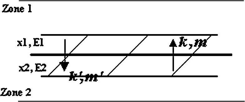
Illustration of two adjacent fishing zones with a small width in the sea.

We suppose that two processes occur at two different time scales. At the fast time scale, the total stock and the total fishing effort are constant. Thus, the fast part of the model only describes the displacement of fish and vessels between the two zones.

At the slow time scale, the total fish stock and the total fishing effort are not constant. Regarding fish stocks, their evolution, in each specific zone, is represented by the stock-effort Schäefer model, also called Graham–Schäefer model (see Schäefer [17]): the growth of the fish population according to the logistic model and its decrease due to the harvested quantity $q_{i} E_{i} x_{i}$ .

Concerning the fishing effort, it is assumed to vary with respect to the investment proportion of the fishing revenue. That means that the fleet owners will invest (or not), with respect to their revenues. Note that the revenue, in the model, is the difference between the income and the cost

We assume that unit prices and unit costs are constant. This is a simplifying assumption as prices could, for example, depend on the abundance of fish available on the market at time t, see Allen and McGlade [1] and Clark [4]. We would like to investigate this process in a future contribution.

According to previous assumptions, the complete system, at the fast time scale τ with respect to t (see Mchich et al. [9,10]), reads as follows:

{\begin{matrix} \frac{d x_{1}}{d τ} = (k x_{2} - k^{'} x_{1}) + ɛ [r_{1} x_{1} (1 - \frac{x_{1}}{K_{1}}) - q_{1} E_{1} x_{1}] \\ \frac{d x_{2}}{d τ} = (k^{'} x_{1} - k x_{2}) + ɛ [r_{2} x_{2} (1 - \frac{x_{2}}{K_{2}}) - q_{2} E_{2} x_{2}] \\ \frac{d E_{1}}{d τ} = (m E_{2} - m^{'} E_{1}) + ɛ α (t) E_{1} (p_{1} q_{1} x_{1} - c_{1}) \\ \frac{d E_{2}}{d τ} = (m^{'} E_{1} - m E_{2}) + ɛ α (t) E_{2} (p_{2} q_{2} x_{2} - c_{2}) \end{matrix}

(2.1)

where

r_{i}

and

K_{i} (i = 1, 2)

represent, respectively, the intrinsic growth rate and carrying capacity of the stock in zone i. Patches have distinct characteristics, so we suppose that parameters

r_{1}

and

r_{2}

are different.

The catchability coefficient of the fleet on zone i $(i = 1, 2)$ is $q_{i}$ . It is supposed to be constant and, for simplicity of calculations, we also assume $q_{i} = 1 (i = 1, 2)$ .

Parameters $p_{i}$ and $c_{i} (i = 1, 2)$ are, respectively, the unit price of the catch and the unit cost of the fishing effort unit in zone i, and are assumed to be constant. The constant coefficients k and $k^{'}$ represent the fish per capita migration rates from zone 2 to zone 1 and from zone 1 to zone 2, respectively. The corresponding migration coefficients for the fishing efforts m and $m^{'}$ are assumed to be constant.

The function $α (t)$ is regarded as the proportion of the fishing revenue to be invested, with respect to time. We assume that: $0 ⪯ α (t) ⪯ 1$ . We also assume that: $E \in [E_{\min}, E^{\max}]$ . Clark et al. [5] and Touzeau [18] used similar cases where the fishing effort is bounded by two nonvanished values.

We can finally assume that $E_{\min} ⩾ 1$ .

3 Aggregated system and equilibrium points

A simple calculation leads to the following fast equilibria:

{\begin{matrix} x_{1}^{*} = ν_{1} x, & x_{2}^{*} = ν_{2} x \\ E_{1}^{*} = η_{1} E, & E_{2}^{*} = η_{2} E \end{matrix}

(3.1)

where

ν_{1}

and

ν_{2}

represent the fast equilibrium proportions of the stock on each patch, whereas

η_{1}

and

η_{2}

admit the same interpretation for the fishing effort. All these proportions are given by:

{\begin{matrix} ν_{1} = \frac{k}{k + k^{'}}, & ν_{2} = \frac{k^{'}}{k + k^{'}} \\ η_{1} = \frac{m}{m + m^{'}}, & η_{2} = \frac{m^{'}}{m + m^{'}} \end{matrix}

(3.2)

Now, coming back to the complete initial system (2.1), we substitute the fast equilibria (3.1) and add the two fish stock and the two fishing effort equations. As

x (t) = x_{1} (t) + x_{2} (t) and

E (t) = E_{1} (t) + E_{2} (t)

one obtains the following system (with respect to slow time scale t) which is called the aggregated model:

{\begin{matrix} \dot{x} (t) = r x (t) (1 - \frac{x (t)}{K}) - q E (t) x (t) \\ \dot{E} (t) = α (t) E (t) (p x (t) - c) \end{matrix}

(3.3)

where:

{\begin{matrix} r = r_{1} ν_{1} + r_{2} ν_{2} \\ K = \frac{r}{\frac{r_{1} ν_{1}^{2}}{K_{1}} + \frac{r_{2} ν_{2}^{2}}{K_{2}}} \\ q = η_{1} ν_{1} + η_{2} ν_{2} \end{matrix}

and

{\begin{matrix} p = η_{1} ν_{1} p_{1} + η_{2} ν_{2} p_{2} \\ c = η_{1} c_{1} + η_{2} c_{2} \end{matrix}

The system (3.3) has 3 equilibrium points: $(0, 0)$ , $(K, 0)$ and $(x^{*}, E^{*})$ , where:

x^{*} = \frac{c}{p} and E^{*} = \frac{r}{q} (1 - \frac{c}{p K})

(3.4)

These points permit us to subdivide the $(x, E)$ -plane into 4 areas as in Fig. 2. This subdivision will be important for the study of the aggregated system stabilizability.

Fig. 2
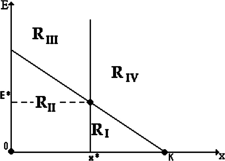
Illustration of nullclines and equilibrium points.

Note that the interesting equilibrium point is $(x^{*}, E^{*})$ , under the condition $p K - c > 0$ . If not, this equilibrium point does not belong to the positive quadrant and no equilibrium point is of interest for the fishing activity. This is a realizable condition. It indicates that the fleets will participate to the fishing activity only if they are ensured with a positive minimal income, i.e. $p K - c > 0$ is a condition which permits the viability of the fishing activity and a positive revenue for the fleets owners.

Note also that the aggregated system (3.3) contains a control function $α (t)$ , in the equation describing the evolution of the total fishing effort. Thus, in the following section, we will study the stabilizability of the system (3.3) in the neighborhood of the interesting equilibrium point $(x^{*}, E^{*})$ .

4 Main results of stabilizability

4.1 Stabilizability

In order to prove that a system:

\dot{x} (t) = f (x (t), u (t))

is globally stabilized, we must prove the existence of a (even discontinuous) feedback

u : R^{n} \to U

, such that the equation:

\dot{x} (t) = f (x, u (x))

is globally asymptotically stable. This returns, in fact, to prove the existence of a smooth Lyapunov function of control

V (x (t))

satisfying the following assumption:

\forall x \neq 0, 〈 \nabla V (x), f (x, u) 〉 < 0

(4.1)

This is a sufficient but not a necessary condition. For more details about the stabilizability concept, see, for example, the works of Clarke [6] and Rifford [16].

Now, we state the following result:

Theorem 4.1

The function

V (x, E) = {(x - x^{*})}^{2} + \frac{K q}{p E_{\min}} {(E - E^{*})}^{2}

(4.2)

where

(x^{*}, E^{*})

is given by (3.4) , is a smooth Lyapunov function of control associated to the system (3.3) .

Moreover, the feedback $\bar{α} (x, E)$ given by:

\bar{α} (x, E) = {\begin{matrix} \frac{E_{\min}}{K} \frac{x}{E} & in R_{I} \\ 0 & in R_{II} \\ \frac{E_{\min}}{K} \frac{x}{E} & in R_{III} \\ 0 & in R_{IV} \end{matrix}

(4.3)

where areas

R_{I}

R_{II}

R_{III}

and

R_{IV}

are given byFig. 2, ensures that in each area of the

(x, E)

-plane, the condition(4.1)is satisfied, which will ensure (see Theorem 4.2) the system stabilizability.

Proof

Let us consider the function given by (4.2):

V (x, E) = {(x - x^{*})}^{2} + \frac{K q}{p E_{\min}} {(E - E^{*})}^{2}

This function is a $C^{\infty}$ function with respect to $(x, E)$ . Moreover, it is positive definite ( $V (x, E) > 0$ for all $(x, E) \neq (x^{*}, E^{*})$ ), and $\lim_{‖ (x, E) ‖ \to + \infty} V (x, E) = + \infty$ holds.

Furthermore, the function $V (x, E)$ satisfies the condition (4.1); indeed, let us subdivide the $(x, E)$ -plane into 4 areas as given in Fig. 2. Thus, with:

f (x, \bar{α}) = (r x (1 - \frac{x}{K}) - q E x; \bar{α} E (p x - c))

and for all

x \neq x^{*}

and

E \neq E^{*}

, we have:

• In the area

R_{I}

, we have

x > x^{*}

and

E < \frac{r}{q} (1 - \frac{x}{K})

, so we choose

\bar{α} (x, E) = \frac{E_{\min}}{K} \frac{x}{E} .

Indeed,

〈 \nabla V (x), f (x, \bar{α}) 〉 2 (x - x^{*}) [r x (1 - \frac{x}{K}) - q E x] + \frac{2 K q}{p E_{\min}} (E - E^{*}) \bar{α} (x, E) (p x - c) E = 2 x [(x - x^{*}) (r (1 - \frac{x}{K}) - q E) + \frac{q}{p} (E - E^{*}) p (x - \frac{c}{p})] = 2 x (x - x^{*}) [r (1 - \frac{x}{K}) - q E + q (E - \frac{r}{q} (1 - \frac{x^{*}}{K}))] (because x^{*} = \frac{c}{p} and E^{*} = \frac{r}{q} (1 - x^{*} / K)) = 2 x (x - x^{*}) (- \frac{r x}{K} + \frac{r x^{*}}{K}) = - \frac{2 r}{K} x . {(x - x^{*})}^{2} < 0

• In the area $R_{II}$ , we have $x < x^{*}$ and $E < \frac{r}{q} (1 - \frac{x}{K})$ , so we choose
$\bar{α} (x, E) = 0$
Indeed,
$〈 \nabla V (x), f (x, \bar{α}) 〉 2 (x - x^{*}) (r x (1 - \frac{x}{K}) - q E x) + \frac{2 K q}{p E_{\min}} (E - E^{*}) \bar{α} (x, E) (p x - c) E = 2 (x - x^{*}) [x (r (1 - \frac{x}{K}) - q E)] = A . B$
where
$A = 2 (x - x^{*}) < 0 and B = x (r (1 - \frac{x}{K}) - q E) > 0$
So
$〈 \nabla V (x), f (x, \bar{α}) 〉 < 0$
• In the area $R_{III}$ , we have $x < x^{*}$ and $E > \frac{r}{q} (1 - \frac{x}{K})$ , so we choose
$\bar{α} (x, E) = \frac{E_{\min}}{K} \frac{x}{E}$
Indeed:
$〈 \nabla V (x), f (x, \bar{α}) 〉 2 (x - x^{*}) [r x (1 - \frac{x}{K}) - q E x] + \frac{2 K q}{p E_{\min}} (E - E^{*}) \bar{α} (x, E) (p x - c) E = - \frac{2 r}{K} {(x - x^{*})}^{2} < 0$
• In the area $R_{IV}$ , we have $x > x^{*}$ and $E > \frac{r}{q} (1 - \frac{x}{K})$ , so we choose
$\bar{α} (x, E) = 0$
Indeed:
$〈 \nabla V (x), f (x, \bar{α}) 〉 2 (x - x^{*}) (r x (1 - \frac{x}{K}) - q E x) + \frac{2 K q}{p E_{\min}} (E - E^{*}) \bar{α} (x, E) (p x - c) E = 2 (x - x^{*}) [x (r (1 - \frac{x}{K}) - q E)] = A . B$
where
$A = 2 (x - x^{*}) > 0, and$
$B = x (r (1 - \frac{x}{K}) - q E) < 0$
So
$〈 \nabla V (x), f (x, \bar{α}) 〉 < 0 □$

Remark 4.1 (The trajectory behavior when reaching the nullclines)

Let us consider a trajectory starting at an initial point $(x_{0}, E_{0})$ , which is in the area $R_{IV}$ . So, it decreases until reaching the nullcline $x = x^{*}$ . Here, we have: $\dot{x} (t) = r x (1 - \frac{x}{K}) - q E x < 0$ and $\dot{E} (t) = 0$ , so the trajectory continue decreasing and enters into the region $R_{III}$ . Then, the trajectory decreases until reaching the nullcline $E = \frac{r}{q} (1 - \frac{x}{K})$ . On this nullcline, $\dot{x} (t) = 0$ and $\dot{E} (t) < 0$ . So, the trajectory leaves the nullcline by decreasing and enters into the area $R_{II}$ . We can give the same interpretation when the trajectory reaches the nullclines $x = x^{*}$ and $E = \frac{r}{q} (1 - \frac{x}{K})$ , when leaving areas $R_{II}$ and $R_{I}$ , respectively.

Now, we state the following theorem, which ensures the stabilizability of the system (3.3), with the discontinuous feedback $\bar{α} (x, E)$ :

Theorem 4.2

For the Lyapunov function $V (x, E)$ given by (4.2) , and the discontinuous feedback given by (4.3) , associated to the system (3.3) , then this system is globally asymptotically stable near the equilibrium point $(x^{*}, E^{*})$ .

Proof

In order to demonstrate this theorem, we first give some notations, to translate the equilibrium point $(x^{*}, E^{*})$ towards $(0, 0)$ . For that, we set:

X (t) = (x (t), E (t)) and X^{*} = (x^{*}, E^{*})

\bar{f} (X (t), \bar{β} (X)) = f ((x + x^{*}, E + E^{*}), \bar{β} (X))

where

f (x, E) = [r x (t) (1 - \frac{x (t)}{K}) - q E (t) x (t); α (t) E (t) (p x (t) - c)]

and

\bar{β} (X) = \bar{α} (x + x^{*}, E + E^{*})

where

\bar{α} (x, E)

is given by (4.3).

Thus, the problem (3.3) is reduced to the following one:

\dot{X} (t) = \bar{f} (X (t), \bar{β} (X))

(4.4)

with the equilibrium point

X = 0

On the other hand, let us consider the following Lyapunov function associated to the problem (4.4):

\bar{V} (X) = V (x + x^{*}, E + E^{*})

where

V (x, E)

is given by (4.2).

Now, let $X_{0}$ be given, then the system:

{\begin{matrix} \dot{X} (t) = \bar{f} (X (t), \bar{β} (X_{0})), & t ⩾ 0 \\ X (0) = X_{0} \end{matrix}

admits a local solution on

[0, t_{0} [

(thanks to the Cauchy–Lipschitz theorem). Moreover, let us assume that:

\lim_{t \to t_{0}} X (t) = X_{1} < + \infty

so the system:

{\begin{matrix} \dot{X} (t) = \bar{f} (X (t), \bar{β} (X_{1})), t ⩾ t_{0} \\ X (t_{0}) = X_{1} \end{matrix}

admits also a solution on

[t_{0}, t_{1} [

. As a consequence, if the function

X (t)

remains bounded, then we can construct gradually, a global solution of the system (4.4) on

[0, + \infty [

Thus, we must prove that the local solution of the system (4.4) is bounded. Indeed, since $\bar{V}$ satisfies the condition (4.1), we have:

\frac{d}{d t} \bar{V} (X (t)) = {\bar{V}}^{'} (X (t)) \bar{f} (X (t), \bar{β} (X (t))) ⩽ 0

so, the function

t \to \bar{V} (X (t))

is decreasing on

[0, t_{0} [

. If we set

c = \bar{V} (X (0))

, then

X (t) \in E_{c} = {s \in R^{n}, \bar{V} (s) ⩽ c}

The set $E_{c}$ is closed (because $\bar{V}$ is continuous), bounded (thanks to the coercivity of $\bar{V}$ ). This implies that the solution $X (t)$ remains in a compact set. So, this solution is bounded, and we can define $X (.)$ on $[0, + \infty [$ .

Now, we must prove that the solution $X (t)$ of the system (4.4), converges uniformly towards 0. For that, let us set: $V_{\infty} = \lim_{t \to + \infty} \bar{V} (X (t))$ (<∞, because $X (t) \in E_{c}$ ).

Lemma 4.3

$V_{\infty} = 0$ .

Proof

Let us assume that $V_{\infty} > 0$ : then, let $X (t)$ be a solution (in the Euler solutions way) of (4.4), such that: $\lim_{t \to + \infty} X (t) = X_{\infty}$ . So, we necessarily have $\bar{V} (X_{\infty}) = V_{\infty}$ , and thus $V_{\infty} ⩽ \bar{V} (X (t))$ for all $t ⩾ 0$ (because $\bar{V} (X (t))$ is a decreasing function).

Let us consider the function $\tilde{X} (.)$ which is a solution of the following system:

{\begin{matrix} \dot{X} (t) = f (X (t), \bar{β} (X (t))), t ⩾ 0 \\ X (0) = X_{\infty} \end{matrix}

(4.5)

As the function $t \to \bar{V} (\tilde{X} (t))$ is decreasing, we will have (from a time t) $\bar{V} (\tilde{X} (t)) < V_{\infty}$ .

In other words, the solution of the system (4.5), at a given time, enters and remains in the whole set ${s, \bar{V} (s) < V_{\infty}}$ . And thus, from a larger time T, the function $X (t)$ verify:

X (t) \in {s, \bar{V} (s) < V_{\infty}}, \forall t ⩾ T

Then

V_{\infty} = \bar{V} (X_{\infty}) ⩽ \bar{V} (X (t)) < V_{\infty}, for all t ⩾ T

Which is absurd. Thus $V_{\infty} = 0$ , which finishes the demonstration of the lemma. □

So, we finish the proof of the theorem, since $V_{\infty} = 0$ implies that $\lim_{t \to + \infty} X (t) = 0$ . □

4.2 Finite time strategy

The feedback defined in the preceding section stabilizes the system in infinite time. But it is more practical and realistic, for the coastal state and the fleets owners, to describe a strategy which will accelerate the procedure of convergence of the system towards a small neighborhood of the equilibrium point, in a finite time (see Fig. 3).

Fig. 3
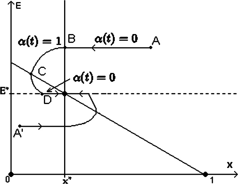
A finite time equilibrium strategy. Data have been chosen (in the case of the trajectory $A \to B \to C \to D \to (x^{*}, E^{*})$ ) as: r=0.5, K=1, q=0.5, p=0.4, c=0.2.

Thus, let us consider a trajectory starting at an initial point A located in the area $R_{IV}$ . We have $x > x^{*}$ and $E > E^{*}$ , so, we take $α (t) = 0$ . Thus, the fishing effort remains constant while the stock decreases. So, the trajectory decreases horizontally until reaching a point B on the line $x = x^{*}$ . Next, when passing the point B, we change the strategy by taking $α (t) = 1$ , in order to keep $E (t)$ and $x (t)$ decreasing, until reaching the nullcline $E = \frac{r}{q} (1 - \frac{x}{K})$ at a point C. When passing this last point, E continues decreasing while x starts increasing, until reaching a point D on the line $E = E^{*}$ . Next, we choose the feedback as $α (t) = 0$ , and so one remains on the line $E = E^{*}$ until reaching the equilibrium point.

One can also start from an initial point $A^{'}$ in the area $R_{II}$ , and make a similar reasoning to reach the equilibrium point $(x^{*}, E^{*})$ .

4.3 Extension of the results

In order to avoid any overexploitation of the fishery, we think that it will be better for a coastal state to intervene directly in the fishing activity, by imposing a reduction or an increase in the fishing efforts.

This can be done by considering, in systems (2.1) and (3.3), the investment proportion $α (t)$ as a control function, bounded between −1 and 1. A negative control can be seen in this case as a reduction (by the decision maker, which is the coastal state in our case) of boats fish capacity (number of boats, technical characteristics.. ). Note that a negative investment was already used in preceding works, see, for example, Clark [4] and Clark et al. [5].

Thus, concerning the evolution of fishing efforts at the slow time, they increase or decrease with respect to the investment rate of the fishing revenue, if the revenue of the fishery and the investment rate are positive or negative. That means that the fleet owners are obliged to invest or disinvest, with respect to their incomes, a part of their revenue to increase or reduce their fishing efforts (number of boats, efficiency, ...).

From a mathematical point of view, the results already obtained in the preceding sections remain valid, one could even find another feedback (for the stabilizability) which is negative in some areas. We think that this can also be interesting in the case of the study of the feedback optimality, or in the case where a coastal state has to manage between a national and a foreign fleets. We hope to investigate this way in forthcoming works.

We state a result for a negative feedback:

Theorem 4.4

The function

V (x, E) = {(x - x^{*})}^{2} + \frac{K q}{p E_{\min}} {(E - E^{*})}^{2}

(4.6)

where

(x^{*}, E^{*})

is given by (3.4) , is a smooth Lyapunov function of control associated to the system (3.3) .

Moreover, the feedback $\bar{α} (x, E)$ given by:

\bar{α} (x, E) = {\begin{matrix} \frac{E_{\min}}{K} \frac{x}{E} & in R_{I} \\ \frac{E - E^{*}}{E} & in R_{II} \\ \frac{E_{\min}}{K} \frac{x}{E} & in R_{III} \\ \frac{E^{*} - E}{E} & in R_{IV} \end{matrix}

(4.7)

where areas

R_{I}

R_{II}

R_{III}

and

R_{IV}

are given byFig. 2, ensures that in each area of the

(x, E)

-plane, the condition(4.1)is satisfied. And the system(3.3)is globally asymptotically stable, near the equilibrium point

(x^{*}, E^{*})

Remark 4.2

Similarly to some analysis concerning a negative control given by Clark [4] and Clark et al. [5], we analyze the results of our model with negative control. We notice that a problem can occur in the case where $E (p x - c) < 0$ , which implies a negative income. In this case, if one imposes a control $α (t) < 0$ , which implies an investment withdrawal, then $\dot{E} (t) = α (t) E (p x - c)$ becomes positive, which implies an increase in the number of boats. And this can appear contradictory.

However, we suggest in this case two different interpretations. The first one is that the control can be regarded as a subsidy from the coastal state to the fleets owners, in order to increase their fishing efforts. The second one is that one could see in the investment withdrawal a reduction of the number of boats, which will act positively on their efficiency, and in this case, we can interpret the fishing efforts as the efficiency of the fishing boats. Note that the fishing effort of a fleet can even be interpreted as the number of boats, days of fishing, boats efficiency... (for this, one can refer to the web-site of the FAO organization [19]).

Proof of Theorem 4.1

In areas $R_{I}$ and $R_{III}$ , the proof remains the same as in Theorem 4.1. On the other hand, we have:

• In the area $R_{II}$ , we have $x < x^{*}$ and $E < \frac{r}{q} (1 - \frac{x}{K})$ , so we choose
$\bar{α} (x, E) = \frac{E - E^{*}}{E}$
Indeed,
$〈 \nabla V (x), f (x, \bar{α}) 〉 2 (x - x^{*}) (r x (1 - \frac{x}{K}) - q E x) + \frac{2 K q}{p E_{\min}} (E - E^{*}) \bar{α} (x, E) (p x - c) E = 2 (x - x^{*}) [x (r (1 - \frac{x}{K}) - q E) + \frac{K q}{E_{\min}} {(E - E^{*})}^{2}] = A [B + C],$
where
$A = 2 (x - x^{*}) < 0$
$B = x (r (1 - \frac{x}{K}) - q E) > 0$
$C = \frac{K q}{E_{\min}} {(E - E^{*})}^{2} > 0$
So
$〈 \nabla V (x), f (x, \bar{α}) 〉 < 0$
• In the area $R_{IV}$ , we have $x > x^{*}$ and $E > \frac{r}{q} (1 - \frac{x}{K})$ , so we choose
$\bar{α} (x, E) = \frac{E^{*} - E}{E}$
Indeed:
$〈 \nabla V (x), f (x, \bar{α}) 〉 2 (x - x^{*}) (r x (1 - \frac{x}{K}) - q E x) + \frac{2 K q}{p E_{\min}} (E - E^{*}) \bar{α} (x, E) (p x - c) E = 2 (x - x^{*}) [x (r (1 - \frac{x}{K}) - q E) - \frac{K q}{E_{\min}} {(E - E^{*})}^{2}] = A [B + C]$
where
$A = 2 (x - x^{*}) > 0$
$B = x (r (1 - \frac{x}{K}) - q E) < 0$
$C = - \frac{K q}{E_{\min}} {(E - E^{*})}^{2} < 0$
Finally, for the global asymptotical stability, the proof remains the same as the one of Theorem 4.2. □

Remark 4.3

For the finite time strategy, we can describe it as follows (see Fig. 4).

Fig. 4
A finite time equilibrium strategy. Data have been chosen (in the case of the trajectory $A \to B_{2} \to C \to D \to (x^{*}, E^{*})$ ) as: r=0.5, K=1, q=0.5, p=0.4, c=0.2.

Thus, let us consider a trajectory starting at an initial point A located in the area $R_{IV}$ . We have $x > x^{*}$ and $E > E^{*}$ , so, we take $α (t) = - 1$ , thus, we have two cases:

(1) The trajectory decreases until reaching the line $E = E^{*}$ at a point $B_{1}$ . In this case, we choose the feedback as $α (t) = 0$ , and one remains on this line until reaching the equilibrium point $(x^{*}, E^{*})$ .
(2) The trajectory decreases until reaching the nullcline $x = x^{*}$ at a point $B_{2}$ . Next, when passing the point $B_{2}$ , we change the strategy by taking $α (t) = 1$ , in order to keep $E (t)$ and $x (t)$ decreasing, until reaching the nullcline $E = \frac{r}{q} (1 - \frac{x}{K})$ at a point C. When passing this last point, E continue decreasing while x start increasing, until reaching a point D on the line $E = E^{*}$ . Next, we choose the feedback as $α (t) = 0$ , and so one remains on the line $E = E^{*}$ until reaching the equilibrium point.

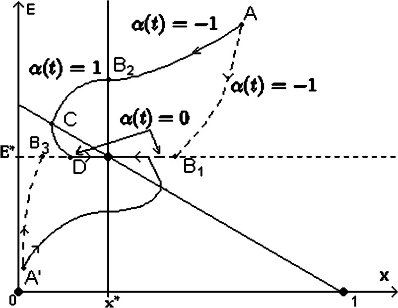
One can also start from an initial point $A^{'}$ in the area $R_{II}$ , and make a similar reasoning to reach the equilibrium point $(x^{*}, E^{*})$ .

5 Stabilizability in the case of fish stock-dependent migration rates

In Mchich et al. [10], we built and studied a model which exhibits, under some conditions, a stable limit cycle. The complete system read as follows:

{\begin{matrix} \frac{d x_{1}}{d τ} = (k x_{2} - k^{'} x_{1}) + ɛ [r_{1} x_{1} (1 - \frac{x_{1}}{K_{1}}) - E_{1} x_{1}] \\ \frac{d x_{2}}{d τ} = (k^{'} x_{1} - k x_{2}) + ɛ [r_{2} x_{2} (1 - \frac{x_{2}}{K_{2}}) - E_{2} x_{2}] \\ \frac{d E_{1}}{d τ} = (m (x_{2}) E_{2} - m^{'} (x_{1}) E_{1}) + ɛ E_{1} (p_{1} x_{1} - c_{1}) \\ \frac{d E_{2}}{d τ} = (m^{'} (x_{1}) E_{1} - m (x_{2}) E_{2}) + ɛ E_{2} (p_{2} x_{2} - c_{2}) \end{matrix}

(5.1)

We had taken the migrations rates as:

m^{'} (x_{1}) = \frac{1}{α x_{1} + α_{0}} and m (x_{2}) = \frac{1}{β x_{2} + α_{0}}

and the aggregated system read as follows:

{\begin{matrix} \dot{x} (t) = r x (1 - \frac{x}{K}) - q (x) E x \\ \dot{E} (t) = E (p (x) x - c (x)) \end{matrix}

(5.2)

where:

{\begin{matrix} r = r_{1} ν_{1} + r_{2} ν_{2} \\ K = \frac{r}{\frac{r_{1} {(ν_{1})}^{2}}{K_{1}} + \frac{r_{2} {(ν_{2})}^{2}}{K_{2}}} \\ q (x) = ν_{1} η_{1} (x) + ν_{2} η_{2} (x) \end{matrix}

(5.3)

{\begin{matrix} p (x) = p_{1} ν_{1} η_{1} (x) + p_{2} ν_{2} η_{2} (x) \\ c (x) = c_{1} η_{1} (x) + c_{2} η_{2} (x) \end{matrix}

(5.4)

and

{\begin{matrix} ν_{1} = \frac{k}{k + k^{'}}, η_{1} (x) = \frac{α ν_{1} x + α_{0}}{(α ν_{1} + β ν_{2}) x + 2 α_{0}} \\ ν_{2} = \frac{k^{'}}{k + k^{'}}, η_{2} (x) = \frac{β ν_{2} x + α_{0}}{(α ν_{1} + β ν_{2}) x + 2 α_{0}} \end{matrix}

(5.5)

We showed that the aggregated system (5.2) has 3 equilibrium points: $(0, 0)$ , $(K, 0)$ and $(x^{*}, E^{*})$ , where $x^{*} > 0$ and $E^{*} = \frac{r}{q (x^{*})} (1 - \frac{x^{*}}{K})$ .

By setting $τ_{1} = α ν_{1} + β ν_{2}$ and $τ_{2} = α ν_{1}^{2} + β ν_{2}^{2}$ , we showed in [10] that if $2 τ_{2} < τ_{1}$ and $x^{*} < \hat{x} < K$ then $(x^{*}, E^{*})$ belongs to the positive quadrant, is unstable and presents a limit cycle, while $(K, 0)$ is a stable node. We recall that $\hat{E}$ represents the maximum value of the nontrivial x-nullcline and $\hat{x}$ the corresponding fish stock value (see Fig. 5).

Fig. 5
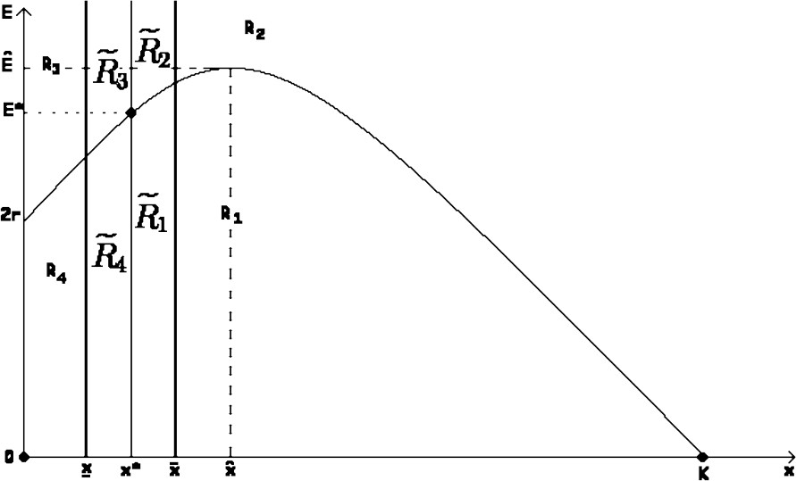
Illustration of nullclines and equilibrium points.

We introduced a control parameter as a term of catchability to avoid this case and to lead the system to the desired stable equilibrium point $(x^{*}, E^{*})$ . However, it is more realistic to control the aggregated system by a control function depending on time. In this section, we analyze this case by studying the following model:

{\begin{matrix} \frac{d x_{1}}{d τ} = (k x_{2} - k^{'} x_{1}) + ɛ [r_{1} x_{1} (1 - \frac{x_{1}}{K_{1}}) - E_{1} x_{1}] \\ \frac{d x_{2}}{d τ} = (k^{'} x_{1} - k x_{2}) + ɛ [r_{2} x_{2} (1 - \frac{x_{2}}{K_{2}}) - E_{2} x_{2}] \\ \frac{d E_{1}}{d τ} = & (m (x_{2}) E_{2} - m^{'} (x_{1}) E_{1}) \\ + ɛ α (t) E_{1} (p_{1} x_{1} - c_{1}) \\ \frac{d E_{2}}{d τ} = & (m^{'} (x_{1}) E_{1} - m (x_{2}) E_{2}) \\ + ɛ α (t) E_{2} (p_{2} x_{2} - c_{2}) \end{matrix}

(5.6)

As in preceding sections, the control function $α (t)$ is regarded as an investment (or investment withdrawal) proportion of the fishing revenue. In this case, the aggregated system reads as follows:

{\begin{matrix} \dot{x} (t) = r x (1 - \frac{x}{K}) - q (x) E x \\ \dot{E} (t) = α (t) E (p (x) x - c (x)) \end{matrix}

(5.7)

with all parameters as in systems (5.3), (5.4) and (5.5).

This system has also 3 equilibrium points: $(0, 0)$ , $(K, 0)$ and $(x^{*}, \frac{r}{q (x^{*})} (1 - \frac{x^{*}}{K}))$ , ( $x^{*} > 0$ ). So, we can subdivide the $(x, E)$ -plan as in Fig. 5.

Note that if $x > x^{*}$ then $p (x) x - c (x) > 0$ . Let $\bar{x} : = x^{*} + ɛ$ where $ɛ ≪ 1$ , and $μ : = p (\bar{x}) \bar{x} - c (\bar{x}) > 0$ . Then for all $x > \bar{x}$ , we have $p (x) x - c (x) > μ$ .

On the other hand, if $x < x^{*}$ then $p (x) x - c (x) < 0$ . So, let $\underset{̲}{x} : = x^{*} - ɛ$ (with $ɛ ≪ 1$ ), and $μ : = p (\underset{̲}{x}) \underset{̲}{x} - c (\underset{̲}{x}) < 0$ . Then for all $x < \underset{̲}{x}$ , we have $p (x) x - c (x) < μ$ .

In the two cases, we have:

\frac{μ}{(p (x) x - c (x))} < 1

Now, we state a theorem for the stabilizability of the aggregated system (5.7):

Theorem 5.1

The function

V (x, E) = \frac{1}{E_{\min}} {(x - x^{*})}^{2} + \frac{K^{2}}{μ E_{\min}^{2}} {(E - E^{*})}^{2}

(5.8)

is a smooth Lyapunov function of control associated to the system (5.7) .

Moreover, the feedback $\bar{α} (x, E)$ given by:

\bar{α} (x, E) = {\begin{matrix} \frac{r μ E_{\min}^{2}}{K^{2}} . \frac{x (x - x^{*})}{(p (x) x - c (x)) E (E^{*} - E)} \\ in R_{1} \\ 0 in R_{2}, R_{4} and {\tilde{R}}_{i} (i = 1, \dots, 4) \\ \frac{μ E_{\min}}{K^{2}} . \frac{q (x) x (x - x^{*})}{(p (x) x - c (x)) (E - E^{*})} \\ in R_{3} \end{matrix}

(5.9)

where areas

R_{i} and {\tilde{R}}_{i} (i = 1, \dots, 4)

are given byFig. 5, ensures that in each area of the

(x, E)

-plane, the condition(4.1)is satisfied. And the aggregated system(5.7)is globally asymptotically stable, near the equilibrium point

(x^{*}, E^{*})

Proof

Let us consider the function given by (5.8):

V (x, E) = \frac{1}{E_{\min}} {(x - x^{*})}^{2} + \frac{K^{2}}{μ E_{\min}^{2}} {(E - E^{*})}^{2}

Furthermore, the function $V (x, E)$ satisfies the condition (4.1); indeed, with

f (x, \bar{α}) = (r x (1 - \frac{x}{K}) - q (x) E x; \bar{α} E (p (x) x - c (x)))

and for all

x \neq x^{*}

and

E \neq E^{*}

, we have:

• In the area

R_{1}

, we have

x > x^{*}

and

E < \frac{r}{q (x)} (1 - \frac{x}{K})

, so we choose

\bar{α} (x, E) = \frac{r μ E_{\min}^{2}}{K^{2}} . \frac{x (x - x^{*})}{(p (x) x - c (x)) E (E^{*} - E)}

Indeed,

〈 \nabla V (x), f (x, \bar{α}) 〉 = \frac{2 (x - x^{*})}{E_{\min}} [r x (1 - \frac{x}{K}) - q (x) E x] + \frac{2 K^{2}}{μ E_{\min}^{2}} (E - E^{*}) \bar{α} (x, E) E (p (x) x - c (x)) = \frac{2 x (x - x^{*})}{E_{\min}} [r - \frac{r x}{K} - q (x) E] - 2 r x (x - x^{*}) = \frac{2 x (x - x^{*})}{E_{\min}} [- r \frac{x}{K} - q (x) E + (r - E_{\min} r)] < 0

because

x - x^{*} > 0

and

E_{\min} ⩾ 1

which implies that

r - E_{\min} r ⩽ 0

Finally, for the global asymptotical stability of the aggregated system (5.7) near the equilibrium point $(x^{*}, E^{*})$ , the proof remains the same as the one of Theorem 4.2. □

6 Conclusion

In this paper, we generalized our previous works (Mchich et al. [9,10]), where we studied the stability of some bioeconomical models. In some cases, we found the existence of a stable limit cycle. This is a critical situation, as it does not permit a satisfied durability of the fishing activity. Indeed, large periods (of time) with small fish stocks and external fluctuations could lead to the extinction of the fish stock.

In order to avoid such situations, in this work, we introduce a control function depending on time, which is considered as an investment proportion of the fishing revenue, into the fishing efforts equations. We construct Lyapunov functions and feedbacks to show that any solution of the aggregated systems, converges in an uniform way, towards the desired equilibrium point. This means that we can find a feedback, which allows us to avoid the undesired cases.

An important limitation of our models comes from the fact that we consider only two fishing zones. The application of our results would be more interesting in the case of N fishing zones ( $N > 2$ ). Also, it would be useful to confront our models with real data, and to try to validate our analytic results. Thus, the model could be concretely applied to the Moroccan coast which is 3500 km long with several important fishing zones (see Fig. 6). Fishing vessels can move from north to south to exploit different fish species, and also they can operate either on coastal or high sea fisheries. Fish stocks could be considered with respect to different species, ages and various aspects intervening in fisheries (see Fig. 6).

Fig. 6
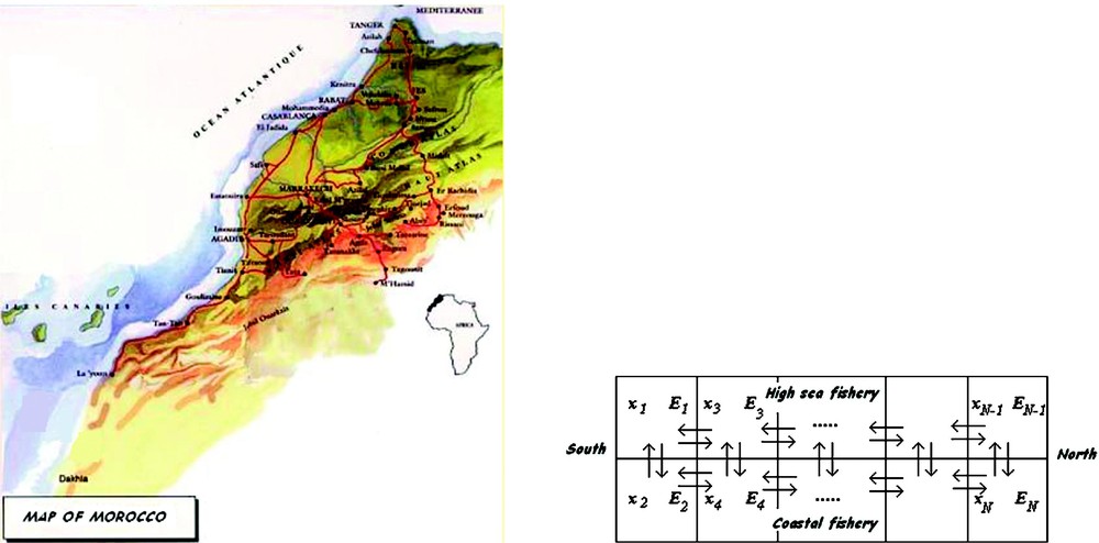
The first figure represents the map of Morocco and the second one illustrates a subdivision of a fishery into N zones.

Another situation worth to be considered is that of different control functions for each fishing fleet. This would permit, for example, in the case of national and foreign fleets, to have different controls for each fleet.

Economically, we think that the model would be more interesting if we would consider a fishery management problem. It would consist on maximizing the fishing revenue, with a spatial distribution of the state variables (fish stocks and fishing efforts) according to adequate boundary conditions. One can see for example the model used by Neubert in [14].

The variety of the control choice would permit to take into account some economical and social problems of the management of various fisheries. The results obtained could be used as a platform for the elaboration of a plan for the management of different kinds of fisheries, particularly, the repartition between the coastal and the high sea fisheries.

Acknowledgments

We thank the anonymous referee for the valuable comments that allowed us to improve the manuscript.

Bibliographie

[1] P.M. Allen; J.M. McGlade Dynamics of discovery and exploitation: the case of the Scotian shelf groundfish fisheries, Can. J. Fish. Aquat. Sci., Volume 43 (1986), pp. 1187-1200

[2] P.M. Auger; J.-C. Poggiale Emergence of population growth models: fast migration and slow growth, J. Theor. Biol., Volume 182 (1996), pp. 99-108

[3] P.M. Auger; R. Roussarie Complex ecological models with simple dynamics: from individuals to population, Acta Biotheor., Volume 42 (1994), pp. 111-136

[4] C.W. Clark The Optimal Management of Renewable Resources. Mathematical Bioeconomics, Wiley-Interscience, New York, 1990

[5] C.W. Clark; F.H. Clarke; G.R. Munro The optimal exploitation of renewable resource stocks: problems of irreversible investment, Econometrica, Volume 47 (1979) no. 1, pp. 25-47

[6] F.H. Clarke; Yu.S. Ledyaev; R.J. Strem; P.R. Wolenski Nonsmooth Analysis and Optimal Control Theory, Graduate Texts in Mathematics, vol. 178, Springer, Berlin, 1998

[7] N. Fenichel Persistence and smoothness of invariant manifolds for flows, Indiana Univ. Math. J., Volume 21 (1971), pp. 193-226

[8] V. Kaitala; G. Munro The conservation and management of high seas fishery resources under the new law of the sea, Nat. Resour. Model., Volume 10 (1997) no. 2

[9] R. Mchich; P.M. Auger; N. Raïssi The dynamics of a fish stock exploited between two fishing zones, Acta Biotheor., Volume 48 (2000) no. 3–4, pp. 207-218

[10] R. Mchich; P.M. Auger; R. Bravo de la Parra; N. Raïssi Dynamics of a fishery on two fishing zones with fish stock dependent migrations: aggregation and control, Ecol. Model., Volume 158 (2002) no. 1–2, pp. 51-62

[11] R. McKelvey, The North American pacific salmon wars: crafting the treaty of peace, in: D. McDonald, M. McAleer (Eds.), Proc. Int. Congress on Modelling and Simulation, 8–11 December 1997, vol. 4, pp. 1548–1555

[12] J. Michalski; J.-C. Poggiale; R. Arditi; P.M. Auger Macroscopic dynamic effects of migrations in patchy predator–prey systems, J. Theor. Biol., Volume 185 (1997), pp. 459-474

[13] G.R. Munro; R.L. Stokes The Canada–United States Pacific salmon treaty (D. McRae; G. Munro, eds.), Canadian Oceans Policy: National Strategies and the New Law of the Sea, University British Columbia Press, Vancouver, Canada, 1989 (pp. 17–35)

[14] M.G. Neubert Marine reserves and optimal harvesting, Ecol. Lett., Volume 6 (2003), pp. 843-849

[15] J.C. Poggiale, Applications des variétés invariantes à la modélisation de l'hétérogénéité en dynamique des populations. PhD thesis, ‘université de Bourgogné’, Dijon, France, 1994

[16] L. Rifford, Problèmes de stabilisation en théorie du contrôle. PhD thesis, Institut Girard-Desargues, University of Lyon-1, France, 2000

[17] M.B. Schäefer Some aspects of the dynamics of populations important to the management of the commercial marine fisheries, Bull. Inter-Am. Trop. Tuna Comm., Volume 1 (1954), pp. 25-26

[18] S. Touzeau, Modèle de contrôle en gestion des pêches, PhD thesis, University of Nice–Sophia-Antipolis, France, 1997

[19] http://www.fao.org/fi/struct/fip.asp

[20] http://www.ifremer.fr/drogm/zee/

[21] http://www.maritimeboundaries.com