Optimal strategy for structured model of fishing problem

Mounir Jerry; Nadia Raïssi

doi:10.1016/j.crvi.2004.10.016

Biological modelling / Biomodélisation

Optimal strategy for structured model of fishing problem
[Stratégie optimale d'un problème de pêche basé sur un modèle structuré]

Présenté par : Pierre Auger

Mounir Jerry ¹ ; Nadia Raïssi ¹

¹ Laboratoire SIANO, Département de mathématiques et d'informatique, université Ibn Tofail, faculté des sciences, BP 133, Kénitra, Maroc

Comptes Rendus. Biologies, Volume 328 (2005) no. 4, pp. 351-356.

Résumés

Anglais
Français

In this work we study a structured fishing model, basically displaying the two stages of the ages of a fish population, which are in our case juvenile, and adults. We associate to this model the maximization of the total discounted net revenues derived by the exploitation of the stock. The exploitation strategy of the optimal control problem is then developed and presented.

Ce travail consiste en l'étude d'un modèle structuré mettant en évidence les différents stades d'âge du stock, en l'occurrence juvénile et adulte. Nous associons à ce modèle la maximisation du total escompté du revenu net généré par l'exploitation du stock. La stratégie d'exploitation du problème de contrôle optimal est recherché.

Métadonnées

Reçu le : 2004-04-26
Accepté le : 2004-11-19
Publié le : 2005-01-29

PMID

DOI : 10.1016/j.crvi.2004.10.016

Keywords: Structural model, Global model, Fishing effort, Optimal strategy, Maximum principle, Recruitment
Mot clés : Modèles structuraux, Modèles globaux, Effort de pêche, Stratégie optimale, Principe de maximum, Recrutement

Affiliations des auteurs :

Mounir Jerry ¹ ; Nadia Raïssi ¹

¹ Laboratoire SIANO, Département de mathématiques et d'informatique, université Ibn Tofail, faculté des sciences, BP 133, Kénitra, Maroc

@article{CRBIOL_2005__328_4_351_0,
     author = {Mounir Jerry and Nadia Ra{\"\i}ssi},
     title = {Optimal strategy for structured model of fishing problem},
     journal = {Comptes Rendus. Biologies},
     pages = {351--356},
     publisher = {Elsevier},
     volume = {328},
     number = {4},
     year = {2005},
     doi = {10.1016/j.crvi.2004.10.016},
     language = {en},
}

TY  - JOUR
AU  - Mounir Jerry
AU  - Nadia Raïssi
TI  - Optimal strategy for structured model of fishing problem
JO  - Comptes Rendus. Biologies
PY  - 2005
SP  - 351
EP  - 356
VL  - 328
IS  - 4
PB  - Elsevier
DO  - 10.1016/j.crvi.2004.10.016
LA  - en
ID  - CRBIOL_2005__328_4_351_0
ER  -

%0 Journal Article
%A Mounir Jerry
%A Nadia Raïssi
%T Optimal strategy for structured model of fishing problem
%J Comptes Rendus. Biologies
%D 2005
%P 351-356
%V 328
%N 4
%I Elsevier
%R 10.1016/j.crvi.2004.10.016
%G en
%F CRBIOL_2005__328_4_351_0

Mounir Jerry; Nadia Raïssi. Optimal strategy for structured model of fishing problem. Comptes Rendus. Biologies, Volume 328 (2005) no. 4, pp. 351-356. doi : 10.1016/j.crvi.2004.10.016. https://comptes-rendus.academie-sciences.fr/biologies/articles/10.1016/j.crvi.2004.10.016/

Version originale du texte intégral

1 Introduction

The models used for resources assessment rarely take into account the total life cycle of an exploited marine population. Often, they only consider the individuals susceptible to exploitation, which constitute the so-called stock. The exploited stock does not contain in general larvas and old fish, because larvas and alevins are too small or absent in the potential fishing zones, and the old fish eventually leave the fishing zones, or become inaccessible to the fleet. But we notice that the fishers do not exclude the fishing of the juvenile, and that it is developing in an alarming way and without control even if there are strict measures that forbid this fishing, therefore to solve this problem, there must take in consideration this fishing with taking in account the juvenile stage in the system that describes the stock evolution.

In building a model of a resource it is necessary to define variables which adequately describe the state of the resource at any time. Such variables are called state variables. For renewable resources they often describe a ‘standing stock’, frequently the number of individuals in a population or the ‘biomass’ of the population. If the age structure, sex ratio, or other population characteristics are important, the model will require more than one state variable. In the literature, models representing the evolution of a stock exploited, are divided in two groups: global models [1–8] and structured models [9–13]; the first one presents the stock as a unique variable, whereas, the second distinguishes between several stages (classes of ages, of size...) of the stock and associates with each one of them a dynamical variable.

So, the global models give a general vision of the stock evolution. But, the responsible authorities of the fishing management may be interested in the impact of certain technical measures like for instance, the reduction of the mesh's fishing nets. The structured models are able to respond to this type of investigations. They permit a qualitative description of the system since they take into account both features: the fish size and the time mechanism of reproduction of the exploited stock.

The objective of this work is to find an optimal strategy of the fishing problem based on a structured model. The case of a dynamics following from a global model is a classic one, and the research of an optimal exploitation policy has been the object of several articles (see, for instance, Clark [1], Clark et al. [2], Jerry and Raïsi [14,15], Raïssi [16]). Section 2 is devoted to the formulation of the fishing problem. In Section 3, we apply the maximum principle to the resulting fishing problem. In Section 4 we present the optimal strategy exploitation.

2 Presentation of the fishing model

Our objective consists on the study of a structured model containing a stage of juvenile. In some previous studies, the recruiting stage is formulated either as a constant or as noise. The restrictive feature of this approach is that the stock – recruitment relationship does not appear. On the other hand, there exist stock – recruitment relationships in literature, for example, the model of Deriso [17], generalized by Schnute [18], Model depositories [19], etc. In this work we are inspired by the models used by Ricker [11,12], Beverton and Holt [9,10], and Touzeau [13] because they are synthetic and mathematically tractable. Even without data on the previous stages of the recruitment, these equations remain a useful tool for the assessment of the stocks [20].

More precisely, our dynamic model is a continuous time model with two states: the juvenile and the adult, where every stage is described by the evolution of its biomass $X_{0}$ and $X_{1}$ , respectively.

{\begin{matrix} {\dot{X}}_{0} = - α X_{0} - m_{0} X_{0} + F_{1} X_{1} - q_{0} E_{0} X_{0} \\ X_{0} (0) = X_{0}^{0} \\ {\dot{X}}_{1} = α X_{0} - m_{1} X_{1} - q_{1} E_{1} X_{1} \\ X_{1} (0) = X_{1}^{0} \end{matrix}

(2.1)

where

E_{i}

and

q_{i}

denote, respectively, the fishing effort and the catchability coefficient for every stage i.

E_{0}

and

E_{1}

are independent, because we consider that we have two fishing fleets which belong to the same decision maker, on the other hand each fleet fishing either juvenile or adults.

Remark 2.1

$X_{0} = 0$ or $X_{1} = 0$ corresponds to the extinction of the species, because if we have $X_{0} = 0$ , according to the first equation of the system (2.1), we will have ${\dot{X}}_{0} = F_{1} X_{1} = 0$ , but $F_{1}$ is a non-null constant, then $X_{1} = 0$ , in the other case, if we have $X_{1} = 0$ , according to the second equation of the system (2.1), we will have ${\dot{X}}_{1} = α X_{0} = 0$ , but α is a non-null constant, then $X_{0} = 0$ .

Each stage i of the stock suffers a mortality rate, due to fishing and natural disaster. The natural mortality incorporates diseases, perturbations generated by the environment and by other species outside the stock, in other words, all factors except the human exploitation and the interactions within the stock. We assume that this mortality is linear (constant rate $m_{i}$ ). The ageing is also supposed to be linear. On the other hand, the passage rate α from the juvenile class to the adult stage is supposed to be constant with respect to time and stage. This means that the time of residence is equal to $\frac{1}{α}$ .

We assume that the laying (eggs) is continuous with respect to time, this assumption constituting a simplification in the model. The species egg laying periods may take place several times per year, even continuously. The number of viable eggs (in the unit of time) introduced in the juvenile stage is given by $F_{1} X_{1}$ , where $F_{1}$ is the mean number of eggs deposited by fertile adult in the unit of time, and $X_{1}$ is the number of adults.

Let us, first note that, according to their definition (mortality rate, fishing effort...), all parameters in the model are nonnegative. For a correct representation of a structured population in the model, we must take into account the recruitment from one class to another, which can be represented by a strictly positive coefficient of passage.

Now assume that the price, $p_{i}$ , of the harvested resource is a fixed constant; furthermore assume that the cost, $c_{i}$ , of a unit of fishing effort is also constant. Then the sole owner's objective is the maximization of the total discounted net revenues derived from exploitation of the resource. We suppose that there exists only one decision-maker of the fishing, who can fish both the juvenile and the adults. If $δ > 0$ is a constant denoting the (continuous) rate of discount, this objective may be expressed as maximizing

\max_{E_{0}, E_{1}} \int_{0}^{\infty} \exp (- δ t) {(p_{0} q_{0} X_{0} (t) - c_{0}) E_{0} (t) + (p_{1} q_{1} X_{1} (t) - c_{1}) E_{1} (t)} d t

(2.2)

actually such that (2.1) is also satisfied, and the controls

E_{0}

E_{1}

are constrained:

0 ⩽ E_{0} (t) ⩽ E_{0}^{\max}, 0 ⩽ E_{1} (t) ⩽ E_{1}^{\max} \forall t ⩾ 0

(2.3)

In this model, the fishing of the juvenile and larvas are not excluded, since we have suppose that the constants $p_{0}$ , $q_{0}$ , and $c_{0}$ are positive. We suppose that:

E_{0}^{\max} ≪ E_{1}^{\max}, p_{0} ≪ p_{1}, q_{0} ≪ q_{1}, c_{0} ≪ c_{1}

(2.4)

It is true that we maximize also the net revenues derived by the exploitation of juvenile (2.2) but the constraints imposed by the problem (2.4) do not encourage this fishing so this revenues is not very significant compared to the revenues generated by the exploitation of adults. With the above formulation, the fishing problem is viewed as an optimal control problem. Our goal consists on the determination of an optimal fishing effort, $({\hat{E}}_{0}, {\hat{E}}_{1})$ , subject to (2.3) and (2.4) such that if $({\hat{X}}_{0}, {\hat{X}}_{1})$ is the corresponding solution of the state system, then $({\hat{E}}_{0}, {\hat{E}}_{1}, {\hat{X}}_{0}, {\hat{X}}_{1})$ maximizes the total discounted net revenues generated by the exploitation of the stock over all admissible processes $(E_{0}, E_{1}, X_{0}, X_{1})$ satisfying (2.1), (2.3) and (2.4).

3 Application of the maximum principle

The data of the model introduced in the previous section satisfies the required standing hypotheses for the application of the maximum principle [21,22]. First we introduce the Hamiltonian:

H (t, E_{0}, E_{1}, X_{0}, X_{1}, R, S) = R (- α X_{0} - m_{0} X_{0} + F_{1} X_{1} - q_{0} E_{0} X_{0}) + S (α X_{0} - m_{1} X_{1} - q_{1} E_{1} X_{1}) + \exp (- δ t) [(p_{0} q_{0} X_{0} - c_{0}) E_{0} + (p_{1} q_{1} X_{1} - c_{1}) E_{1}]

(3.1)

where R and S are additional variables called the adjoint variables. If

({\hat{E}}_{0}, {\hat{E}}_{1})

is an optimal control and

({\hat{X}}_{0}, {\hat{X}}_{1})

is the corresponding response, the maximum principle asserts the existence of adjoint variables

R (t)

and

S (t)

such that the following equations are satisfied, for all t:

{\begin{matrix} - \dot{R} (t) = R (t) (- α - m_{0} - q_{0} {\hat{E}}_{0}) \\ + α S (t) + \exp (- δ t) p_{0} q_{0} {\hat{E}}_{0} \\ - \dot{S} (t) = R (t) F_{1} - S (t) (m_{1} + q_{1} {\hat{E}}_{1}) \\ + \exp (- δ t) p_{1} q_{1} {\hat{E}}_{1} \end{matrix}

(3.2)

If we replace R by $\bar{R} \exp (- δ t)$ , and S by $\bar{S} \exp (- δ t)$ , the associate system (3.2) becomes:

{\begin{matrix} - \dot{\bar{R}} (t) = - \bar{R} (t) (α + δ + m_{0} + q_{0} {\hat{E}}_{0}) \\ + α \bar{S} (t) + p_{0} q_{0} {\hat{E}}_{0} \\ - \dot{\bar{S}} (t) = \bar{R} (t) F_{1} - \bar{S} (t) (m_{1} + δ + q_{1} {\hat{E}}_{1}) \\ + p_{1} q_{1} {\hat{E}}_{1} \end{matrix}

(3.3)

The Hamiltonian become

\begin{matrix} H (t, {\hat{E}}_{0}, {\hat{E}}_{1}, {\hat{X}}_{0}, {\hat{X}}_{1}, \bar{R} (t), \bar{S} (t)) \\ \max_{(E_{0}, E_{1})} {\begin{matrix} [\bar{R} (t) (- α X_{0} - m_{0} X_{0} \\ + F_{1} X_{1} - q_{0} E_{0} X_{0}) \\ + \bar{S} (t) (α X_{0} - m_{1} X_{1} - q_{1} E_{1} X_{1}) \\ + (p_{0} q_{0} X_{0} (t) - c_{0}) E_{0} (t) \\ = \exp (- δ t) + (p_{1} q_{1} X_{1} (t) - c_{1}) E_{1} (t)] \end{matrix}} p.p. \end{matrix}

(3.4)

The Pontryagin's maximum principle provides a necessary optimality condition of $(E_{0}, E_{1})$ . For all t, $({\hat{E}}_{0}, {\hat{E}}_{1})$ must maximize the Hamiltonian. The linearity of the Hamiltonian with respect to the controls leads to a ‘bang–bang’ optimal control: a control that takes on these extreme values is called a bang–bang control

{\begin{matrix} if p_{0} - \frac{c_{0}}{q_{0} X_{0}} - \bar{R} (t) > 0 & then {\hat{E}}_{0} = E_{0}^{\max} \\ if p_{0} - \frac{c_{0}}{q_{0} X_{0}} - \bar{R} (t) < 0 & then {\hat{E}}_{0} = 0 \\ if p_{1} - \frac{c_{1}}{q_{1} X_{1}} - \bar{S} (t) > 0 & then {\hat{E}}_{1} = E_{1}^{\max} \\ if p_{1} - \frac{c_{1}}{q_{1} X_{1}} - \bar{S} (t) < 0 & then {\hat{E}}_{1} = 0 \end{matrix}

(3.5)

However, note that when the switching function $\bar{R} (t) - p_{0} + \frac{c_{0}}{q_{0} X_{0}}$ or $\bar{S} (t) - p_{1} + \frac{c_{1}}{q_{1} X_{1}}$ vanishes, the Hamiltonian becomes independent of $(E_{0}, E_{1})$ , so the maximum principle does not specify the value of the optimal control. The most important case (called the singular case) arises when $\bar{R} (t) - p_{0} + \frac{c_{0}}{q_{0} X_{0}}$ or $\bar{S} (t) - p_{1} + \frac{c_{1}}{q_{1} X_{1}}$ vanishes identically over some time interval of positive length. Establishing the existence of this interval will permit us to identify the following system by deriving these two equations $\bar{R} (t) - p_{0} + \frac{c_{0}}{q_{0} X_{0}} = 0$ and $\bar{S} (t) - p_{1} + \frac{c_{1}}{q_{1} X_{1}} = 0$ :

{\begin{matrix} p_{0} (α + δ + m_{0}) - \frac{c_{0}}{q_{0} X_{0}} (δ + \frac{F_{1} X_{1}}{X_{0}}) \\ - α (p_{1} - \frac{c_{1}}{q_{1} X_{1}}) = 0 \\ δ (p_{1} - \frac{c_{1}}{q_{1} X_{1}}) + m_{1} p_{1} - \frac{α c_{1} X_{0}}{q_{1} X_{1}^{2}} \\ - F_{1} (p_{0} - \frac{c_{0}}{q_{0} X_{0}}) = 0 \end{matrix}

(3.6)

The system (3.6) can admit some solutions, with respect to the parameter values of the problem. Our study will take place in the case where the system (3.6) does not admit any solutions, but with parameter values coming from the literature [13].

The object of the next section is to describe and to prove the optimal strategy of the problem.

4 The optimal strategy

By using the results of the previous section, we are ready to describe definitively the optimal exploitation policy. Now we study the system (3.6) given in the previous section. Let us the following function denote by $Φ_{0} (X_{0}, X_{1})$ , the first equation of system (3.6):

Φ_{0} (X_{0}, X_{1}) = \frac{1}{X_{1}} [p_{0} X_{1} (α + δ + m_{0}) - \frac{c_{0} X_{1}}{q_{0} X_{0}} (δ + \frac{F_{1} X_{1}}{X_{0}}) - α X_{1} (p_{1} - \frac{c_{1}}{q_{1} X_{1}})] = 0

(4.1)

Eq. (4.1) admits two real roots, the first one is positive, and the second is negative, we are interested by the first one:

{\bar{X}}_{1} (X_{0}) = \frac{q_{0} X_{0}^{2}}{2 c_{0} F_{1}} (p_{0} (α + δ + m_{0}) - \frac{δ c_{0}}{q_{0} X_{0}} - α p_{1} + {[{(p_{0} (α + δ + m_{0}) - \frac{δ c_{0}}{q_{0} X_{0}} - α p_{1})}^{2} + \frac{4 α c_{1} c_{0} F_{1}}{q_{1} q_{0} X_{0}^{2}}]}^{1 / 2})

(4.2)

The graph of the function ${\bar{X}}_{1} (X_{0})$ is given by Fig. 1.

Fig. 1
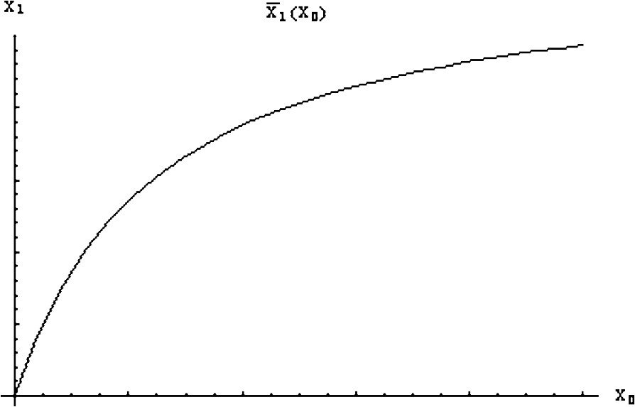
The graph of the function ${\bar{X}}_{1} (X_{0})$ for the following values: α=0.8, $m_{0} = 0.5$ , $m_{1} = 0.2$ , $F_{1} = 0.5$ , $q_{0} = 0.001$ , $q_{1} = 0.8$ , δ=0.2, $c_{0} = 0.08$ , $c_{1} = 0.2$ , $p_{0} = 0.2$ , $p_{1} = 1.2$ .

Consider now the second equation of system (3.6):

Φ_{1} (X_{0}, X_{1}) = \frac{1}{X_{0}} [δ X_{0} (p_{1} - \frac{c_{1}}{q_{1} X_{1}}) + m_{1} p_{1} X_{0} - \frac{α c_{1} X_{0}^{2}}{q_{1} X_{1}^{2}} - F_{1} X_{0} (p_{0} - \frac{c_{0}}{q_{0} X_{0}})] = 0

(4.3)

Eq. (4.3) admits two real roots, the first one is positive, and the second is negative, likewise we are interested by the first root:

{\bar{X}}_{0} (X_{1}) = \frac{q_{1} X_{1}^{2}}{2 α c_{1}} (δ (p_{1} - \frac{c_{1}}{q_{1} X_{1}}) + m_{1} p_{1} - F_{1} p_{0} + {[{(δ (p_{1} - \frac{c_{1}}{q_{1} X_{1}}) + m_{1} p_{1} - F_{1} p_{0})}^{2} + \frac{4 α c_{1} c_{0} F_{1}}{q_{0} q_{1} X_{1}^{2}}]}^{1 / 2})

(4.4)

The graph of the function ${\bar{X}}_{0} (X_{1})$ is given by Fig. 2.

Fig. 2
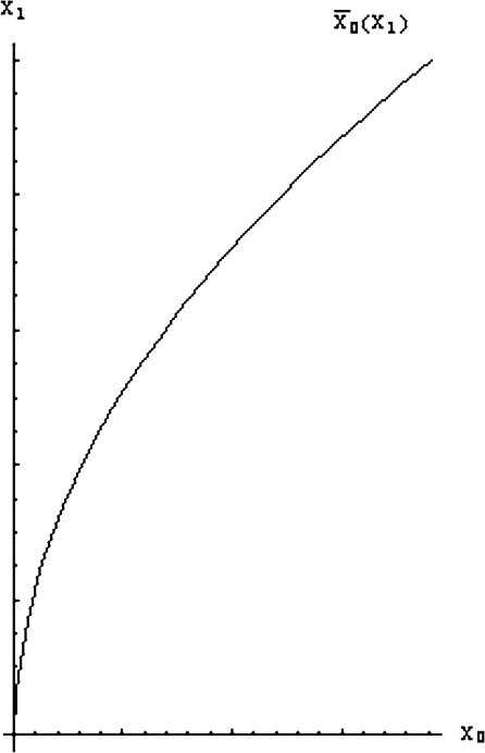
The graph of the function ${\bar{X}}_{0} (X_{1})$ for the following values: α=0.8, $m_{0} = 0.5$ , $m_{1} = 0.2$ , $F_{1} = 0.5$ , $q_{0} = 0.001$ , $q_{1} = 0.8$ , δ=0.2, $c_{0} = 0.08$ , $c_{1} = 0.2$ , $p_{0} = 0.2$ , $p_{1} = 1.2$ .

These parameters are from [13], even if they not correspond at any real stock. Their value depends of the units reserved for the variables of the model, for example, $m_{i}$ depends of the unit of time (year, month...), $F_{1}$ of the number of the stock (in thousand, millions...).

The preceding analysis of the two equations will permit us to prove the two following lemmas:

Lemma 4.1

Consider $(X_{0}, X_{1})$ , if $X_{1} > {\bar{X}}_{1} (X_{0})$ , then the optimal strategy is ${\hat{E}}_{1} = E_{1}^{\max}$ . Otherwise, if $X_{1} < {\bar{X}}_{1} (X_{0})$ , we have ${\hat{E}}_{1} = 0$ .

Lemma 4.2

Consider $(X_{0}, X_{1})$ , if $X_{0} > {\bar{X}}_{0} (X_{1})$ , then the optimal strategy is ${\hat{E}}_{0} = E_{0}^{\max}$ . Otherwise, if $X_{0} < {\bar{X}}_{0} (X_{1})$ , we have ${\hat{E}}_{0} = 0$ .

Taking into account the previous lemmas, we can now describe the optimal strategy that we must follow for any $(X_{0}, X_{1}) \in R^{+} \times R^{+}$ . This optimal strategy is given and illustrate by the following diagram and Fig. 3, respectively:

{\begin{matrix} if X_{0} > {\bar{X}}_{0} (X_{1}) & then {\hat{E}}_{0} = E_{0}^{\max} \\ if X_{0} < {\bar{X}}_{0} (X_{1}) & then {\hat{E}}_{0} = 0 \\ if X_{1} > {\bar{X}}_{1} (X_{0}) & then {\hat{E}}_{1} = E_{1}^{\max} \\ if X_{1} < {\bar{X}}_{1} (X_{0}) & then {\hat{E}}_{1} = 0 \end{matrix}

(4.5)

Fig. 3
Determination of optimal strategy.

We remark that the two curves ${\bar{X}}_{0} (X_{1})$ and ${\bar{X}}_{1} (X_{0})$ do not intersect. if we are above the curve ${\bar{X}}_{0} (X_{1})$ , the juvenile biomass is weak and the adult biomass is large. The optimal control consists of taking $({\hat{E}}_{0}, {\hat{E}}_{1}) = (0, E_{1}^{\max})$ in order to increase the juvenile biomass as fast as possible until the trajectory reaches the area delimited by the two curves and to take as optimal control $({\hat{E}}_{0}, {\hat{E}}_{1}) = (E_{0}^{\max}, E_{1}^{\max})$ . On the other hand, if we are under the curve ${\bar{X}}_{1} (X_{0})$ , the adult biomass is weak and the juvenile biomass is large. The optimal control consists of taking $({\hat{E}}_{0}, {\hat{E}}_{1}) = (E_{0}^{\max}, 0)$ in order to increase the adult biomass as fast as possible until the trajectory reaches the area delimited by the two curves and to take as optimal control $({\hat{E}}_{0}, {\hat{E}}_{1}) = (E_{0}^{\max}, E_{1}^{\max})$ .

It is easy to show that the optimal strategy described above is a bang–bang strategy, and it is very simple to apply because, according to the position of $(X_{0}, X_{1})$ towards two curves $({\bar{X}}_{0} (X_{1}), {\bar{X}}_{1} (X_{0}))$ , on the other hand if we are on one of the two curves, the corresponding optimal strategy is any value of $(E_{0}, E_{1})$ according to the principle of the maximum especially Eq. (3.4). We deduct the feasible optimal policy to our fishing problem.

5 Conclusion

In the previous results [1,9,10,13], the aim was the search of equilibrium points for a structured model and the study of the stability (saddle point, stable and unstable node, stable and unstable focus, center...), but in this work, a structured model is associated with the maximization of a total discounted net revenues derived from exploitation of the resource, and the main objective is to prove the existence of an optimal strategy for the fishing problem. By using the tools of the control theory, in particular, the Pontryagin's maximum principle, we are found the optimal strategy of the fishing problem.

One drawback of the model is that it does not take into consideration any intraspecific competition between species, the competition between the juvenile and the predation of the adults on the small; It is also a structured model only of two states, therefore it would be necessary to see what happens for a model of dimension $N > 2$ , besides we work with constant parameters during the time, but it does not prevent that all results of this work are interesting since they constitute a basis of reflection and they are a valuable data for new works.

Bibliographie

[1] C.W. Clark Mathematical Bioeconomics: The Optimal Management of Renewable Resources, Wiley-Interscience, New York, 1990

[2] C.W. Clark; F.H. Clarke; G.R. Munro Renewable resources stocks, Econometrica, Volume 47 (1979), pp. 25-47

[3] C.W. Clark; G. Munro The economics of fishing and modern capital theory: a simplified approach, J. Environ. Econ. Manage., Volume 2 (1975), pp. 92-106

[4] M. Graham Modern theory of exploiting a fishery, and application to North Sea trawling, J. Cons. Int. Explor. Mer, Volume 37 (1977), p. 3

[5] R. Pearl The Biology of Population Growth, Alfred A. Knoph, New York, 1925

[6] J.J. Pella; P.K. Tomlinson A generalized stock production model, Bull. Inter-American Tropical Tuna Comm., Volume 13 (1969), pp. 421-496

[7] M.B. Schäefer Some aspects of the dynamics of populations important to the management of the commercial marine fisheries, Bull. Inter-American Tropical Tuna Comm., Volume 1 (1954), pp. 25-26

[8] P.F. Verhulst Notice sur la loi que la population suit dans son accroissement, Corr. Math. Phys., Volume 10 (1838), pp. 113-121

[9] R.J.H. Beverton; S.J. Holt On the Dynamics of Exploited Fish Population, Chapman & Hall, London, 1993 (First edition in 1957)

[10] R.J.H. Beverton; S.J. Holt Recruitment and egg-production, On the Dynamics of Exploited Fish Population, Chapman & Hall, London, 1993, pp. 44-67 (Section 6; see [9])

[11] W.E. Ricker Stock and recruitment, J. Fish. Res. Board Can., Volume 11 (1954), pp. 559-623

[12] W.E. Ricker, Handbook of Computations for Biological Statistics of Fish Populations, Bulletin 119, Fisheries Research Board of Canada, 1958

[13] S. Touzeau, Modèle de contrôle en gestion des pêches, thèse, université de Nice–Sophia-Antipolis, 1997

[14] M. Jerry; N. Raïssi A policy of fisheries management based on continuous fishing effort, J. Biol. Syst., Volume 9 (2001) no. 4, pp. 247-254

[15] M. Jerry; N. Raïssi The optimal strategy for a bioeconomical model of a harvesting renewable resource problem, Math. Comput. Modelling, Volume 36 (2002), pp. 1293-1306

[16] N. Raïssi Features of bioeconomics models for the optimal management of a fishery exploited by two different fleets, Nat. Resour. Modeling, Volume 14 (2001) no. 2

[17] R.B. Deriso Harvesting strategies and parameter estimation for an age-structured model, Can. J. Fish. Aquat. Sci., Volume 37 (1980), pp. 268-282

[18] J. Schnute A general theory for analysis for catch and effort data, Can. J. Fish. Aquat. Sci., Volume 42 (1985), pp. 414-429

[19] R. Hilborn; C.J. Walters Quantitative Fisheries Stock Assessment: Choice, Dynamics and Uncertainty, Chapman & Hall, New York, 1992

[20] J.C. Rice, Quantitative methods in recruitment, in: M. Sinclair, J.T. Anderson, M. Chadwick, J. Gagn, W.D. Mckone, J.C. Rice, D. Ware (Eds.), Report from the National Workshop on Recruitment, Held in St. John's, Newfoundland, Canadian Technical Report of Fisheries and Aquatic Sciences, vol. 1626, 1988, pp. 148–164

[21] F.H. Clarke Optimization and Nonsmooth Analysis, Wiley Interscience, New York, 1983

[22] F.H. Clarke, Methods of dynamics and nonsmooth optimization, CBMS-NSF, 1990