Flowering response and crop duration of aromatic rices in diverse environments

S.M. Shahidullah; M.M. Hanafi; M. Ashrafuzzaman; M.A. Salam; A. Khair

doi:10.1016/j.crvi.2009.07.003

Agronomy / Agronomie

Flowering response and crop duration of aromatic rices in diverse environments

Presented by: Philippe Morat

S.M. Shahidullah ^1,² ; M.M. Hanafi ¹; M. Ashrafuzzaman ¹; M.A. Salam ²; A. Khair ³

¹ Institute of Tropical Agriculture, Universiti Putra Malaysia, 43400 UPM Serdang, Selangor, Malaysia
² Bangladesh Rice Research Institute, Gazipur 1701, Bangladesh
³ Department of Botany, Jahangirnagar University, Savar, Dhaka, Bangladesh

Comptes Rendus. Biologies, Volume 332 (2009) no. 10, pp. 909-916.

Abstract

Crop duration of a rice plant, essentially dictated by flowering response, is an important selection criterion. It is determined by the interaction of genotype and environment. A field experiment was conducted with 40 rice genotypes to assess the fluctuation and/or stability of crop duration in a series of 16 environmental conditions. The effects of genotype, environment and all the components of $G \times E$ interaction were highly significant. Among the genotypes Benaful and Gandho kasturi were most sensitive to environmental changes, and indicating lower adaptability over the environments. Crop durations of 17 genotypes were comparatively stable against environmental changes. Four genotypes viz. Basmati PNR346, BR28, Neimat and Sarwati showed only nonlinear sensitivity and thus unpredictable fluctuation. Seventeen genotypes indicated average stability over the environments. The AMMI analysis identified Badshabhog, Basmati Tapl-90, Bhog ganjia, BR38, Elai, Jata katari and Radhuni pagal as most stable genotypes over the environment series. It also advocated three comparatively stable environments for all the genotypes.

Supplementary Materials:
Supplementary material for this article is supplied as a separate file:

mmc1.pdf

Metadata

Received: 2009-05-29
Accepted: 2009-07-18
Published online: 2009-08-19

PMID

DOI: 10.1016/j.crvi.2009.07.003

Keywords: Aromatic rice, Flowering response, Crop duration, AMMI analysis, $ \text{G}\times \text{E}$ interaction

Author's affiliations:

S.M. Shahidullah ^{1, 2}; M.M. Hanafi ¹; M. Ashrafuzzaman ¹; M.A. Salam ²; A. Khair ³

¹ Institute of Tropical Agriculture, Universiti Putra Malaysia, 43400 UPM Serdang, Selangor, Malaysia
² Bangladesh Rice Research Institute, Gazipur 1701, Bangladesh
³ Department of Botany, Jahangirnagar University, Savar, Dhaka, Bangladesh

@article{CRBIOL_2009__332_10_909_0,
     author = {S.M. Shahidullah and M.M. Hanafi and M. Ashrafuzzaman and M.A. Salam and A. Khair},
     title = {Flowering response and crop duration of aromatic rices in diverse environments},
     journal = {Comptes Rendus. Biologies},
     pages = {909--916},
     publisher = {Elsevier},
     volume = {332},
     number = {10},
     year = {2009},
     doi = {10.1016/j.crvi.2009.07.003},
     language = {en},
}

TY  - JOUR
AU  - S.M. Shahidullah
AU  - M.M. Hanafi
AU  - M. Ashrafuzzaman
AU  - M.A. Salam
AU  - A. Khair
TI  - Flowering response and crop duration of aromatic rices in diverse environments
JO  - Comptes Rendus. Biologies
PY  - 2009
SP  - 909
EP  - 916
VL  - 332
IS  - 10
PB  - Elsevier
DO  - 10.1016/j.crvi.2009.07.003
LA  - en
ID  - CRBIOL_2009__332_10_909_0
ER  -

%0 Journal Article
%A S.M. Shahidullah
%A M.M. Hanafi
%A M. Ashrafuzzaman
%A M.A. Salam
%A A. Khair
%T Flowering response and crop duration of aromatic rices in diverse environments
%J Comptes Rendus. Biologies
%D 2009
%P 909-916
%V 332
%N 10
%I Elsevier
%R 10.1016/j.crvi.2009.07.003
%G en
%F CRBIOL_2009__332_10_909_0

S.M. Shahidullah; M.M. Hanafi; M. Ashrafuzzaman; M.A. Salam; A. Khair. Flowering response and crop duration of aromatic rices in diverse environments. Comptes Rendus. Biologies, Volume 332 (2009) no. 10, pp. 909-916. doi : 10.1016/j.crvi.2009.07.003. https://comptes-rendus.academie-sciences.fr/biologies/articles/10.1016/j.crvi.2009.07.003/

Version originale du texte intégral

1 Introduction

Of all the factors that affect agricultural productivity, the most powerful, and at the same time least modifiable, is the climate [1]. The phenotypic expression of a crop is the reflection of combined effect of genotype and environment. The phenotypic responses to changes in environment are not the same for all genotypes and the consequences of variation in genotypes are dependent on environment. This inter-play in effect of genetic and non-genetic components on phenotypic expression of a genotype is what we call genotype–environment interaction [2]. Better understanding of genotype–environment interaction is a basis for determining crop breeding strategies and provides useful information to identify stable genotypes over a range of environments [3]. Therefore, determination of the nature of genotype and environmental variations present in the plant characters and its magnitude are essential.

The geographical distribution of rice growing areas in different parts of the world reveals that rice is cultivated in the most diverse conditions, from 50° N to 35° S [4]. Adaptability of the rice plant to the environment is determined by its morphology and metabolic activity, which may vary according to the variety and growth stage. Differences in the metabolic pattern insure the pliability of adaptation and are reflected ultimately in the differences in morphological appearance of the plant as a whole [5]. Two types of adaptations are recognized. Agronomically, the wide adaptability of a rice variety refers to its high grain yield performance over diverse climatic conditions [6,7]. Specific adaptability is the ability of the rice plant to adjust to a specific adverse environmental condition e.g. deep water, salinity, drought, cold, etc.

Flowering response of a rice plant is the key indicator of crop duration. The subsequent ripening phase is thought to be of comparatively uniform extent of around 30 days [8]. Crop duration of rice cultivars determine their yield potential, local agronomic suitability and ability to escape from drought and natural hazards [9,10]. In irrigated systems, crop duration determines the calendar options for multiple rice cropping and intensified crop rotation [11,12]. Food crisis/availability and seasonal labour use pattern are also considerable issues for crop duration and planting dates. However, crop duration is interactively determined by the genotype and the environment [13].

Aromatic rices, though constitute a small group of rice in the consideration of consumption; it is a special group of rice that is regarded as best in quality [14]. Bangladesh (22–27° N, 88–93° E) has a stock of above 7000 rice germplasm of which around 100 are of aromatic type [15,16]. Aromatic rices are normally transplanted in rainy season (July–August) in Bangladesh and most of them are popularly grown in specific location. In Boro season (November–May), rice plant receives more solar energy because of clear sunshine in longer growth duration, and rationalize a possibility of higher yield. The increasing temperature during ripening period in this season may hamper aroma in kernel. However, obviously genotypic responses in this concern will be different. Higher yield with even mild aroma in some cultivars in Boro season may open a new avenue for increased aromatic rice production. Many workers have performed stability analysis with local and high yielding varieties of rice. But $G \times E$ analysis for crop duration of aromatic rices has not yet been done. However, very limited quantitative data are available on genotype × environment ( $G \times E$ ) interactions of phenological characters and $G \times E$ analysis for crop duration of aromatic rice. Therefore, this study was undertaken to observe the $G \times E$ interaction for crop duration; and to determine the suitability of aromatic rice genotypes over the locations and growing seasons.

2 Materials and methods

2.1 Identity of the genotypes and general experimental details

The experiment was conducted in 2004–2005. A total of 40 rice germplasm composed of 32 local aromatic, five exotic and three non-aromatic rice varieties as standard checks, were selected for this research (Table 1). Among the three non-aromatic varieties, BR28 was a modern Boro, BR39 was a modern T. Aman variety and the third one, Nizersail was used as a standard photoperiod sensitive genotype [17]. Exotic genotypes were collected from Pakistan (Basmati PNR346), Nepal (Sarwati and Sugandha-1) and Iran (Khazar and Neimat). The rest of the rice genotypes represented their distribution throughout Bangladesh. Forty rice genotypes formed the treatment variables and were assigned randomly to each unit plot of $5 m \times 2 m$ dimension. Thirty-day-old seedlings were transplanted in three sets of Aman season and 45 day-old seedlings in Boro season with a spacing of $20 cm \times 20 cm$ . A fertilizer rate of 25–35–10–3 kg ha⁻¹ of P–K–S–Zn in the form of triple super phosphate, muriate of potash, gypsum and zinc sulfate, respectively, was applied as basal dose at final land preparation. Because of wide genotypic variation in phenological development and yield potential, varieties differed enormously in attaining panicle initiation (PI) stage and in the requirement of nutrient elements. For this reason, nitrogen was top-dressed as urea in 2–3 splits to the contrary of a common practice with fixed dose and time routine. The amount of urea and time of application were determined with the help of a leaf colour chart [18]. Crop duration was counted as the time interval from the day of seed bed sowing to the day of 50% flowering.

Sl#	Genotype	Mean	$P_{i}$	$b_{i}$	$S_{d i}^{2}$
V1	Badsha bhog Tapl-63	108.3	−0.18	1.00	5.55
V2	Baoi jhak	105.2	−3.28	0.95	11.78
V3	Basmati Tapl-90	104.3	−4.20	1.00	7.14
V4	Basmati PNR 346	98.2	−10.26	0.98	36.93^∗
V5	Begun bichi	104.7	−3.78	0.91	11.25
V6	Benaful	111.1	2.64	1.21^∗	10.87
V7	Bhog ganjia	106.6	−1.86	1.02	3.81
V8	BRRIdhan28	96.2	−12.32	0.94	45.97^∗
V9	BRRIdhan38	110.2	1.72	0.84^∗	14.64
V10	BRRIdhan39	102.7	−5.80	0.93	12.03
V11	Chinigura	108.2	−0.26	0.99	12.08
V12	Chinikani	110.6	2.09	0.80^∗	9.02
V13	Darshal	111.0	2.53	0.80^∗	6.97
V14	Doiar guro	111.2	2.68	0.80^∗	6.23
V15	Elai	110.1	1.61	1.02	7.72
V16	Gandho kasturi	166.2	57.68	${4.30}^{* *}$	${558.79}^{* *}$
V17	Gandhoraj	107.7	−0.84	0.86^∗	19.45
V18	Hatisail Tapl-101	107.9	−0.61	0.92	17.04
V19	Jamai sohagi	105.6	−2.93	0.94	22.90
V20	Jata katari	105.8	−2.72	0.93	8.14
V21	Jesso balam Tapl-25	107.0	−1.47	0.87^∗	5.35
V22	Jira katari	107.4	−1.11	0.89^∗	5.92
V23	Kalijira Tapl-73	113.5	5.01	0.78^∗	24.77
V24	Kalomai	106.3	−2.22	0.92	10.37
V25	Kamini soru	105.7	−2.80	0.88^∗	6.70
V26	Kataribhog	105.4	−3.14	0.91	9.26
V27	Khazar	105.4	−3.05	0.86^∗	30.68^∗
V28	Laljira Tapl-130	110.5	2.01	0.85^∗	28.77
V29	Niemat	102.0	−6.51	0.95	${68.19}^{* *}$
V30	Nizersail	109.9	1.39	1.08	24.07
V31	Philippine katari	105.2	−3.28	0.96	9.43
V32	Premful	106.6	−1.93	0.84^∗	1.83
V33	Radhuni pagal Tapl-77	115.1	6.64	0.82^∗	10.71
V34	Rajbhog	110.6	2.14	0.85^∗	12.51
V35	Sai bail	106.9	−1.59	0.94	7.59
V36	Sakkor khora	108.8	0.28	0.86^∗	8.02
V37	Sarwati	104.5	−4.01	0.93	35.08^∗
V38	Sugandha-1	103.3	−5.16	0.89^∗	29.73^∗
V39	Tilkapur	108.4	−0.14	0.88^∗	17.54
V40	Ukni madhu	105.4	−3.11	0.91	11.30

2.2 Identity of the environments

The four locations were:

B = Benarpota Farm, BRRI Regional Station, Satkhira (22.72° N, 89.08° E).

C = Charchandia Farm, BRRI Regional Station, Sonagazi, Feni (22.84° N, 91.39° E).

D = Domar Seed Production Farm, BADC, Sonaroy, Domar, Nilphamari (26.10° N, 88.84° E).

H = Headquarter Farm, Bangladesh Rice Research Institute (BRRI), Gazipur (24.00° N, 90.42° E).

Seed sowing was done in four dates. Three dates were in T. Aman (with an interval of 20 days) and one date was in Boro season.

1 = 1st planting in T. Aman (sowing in seedbed on 16th July 2004).

2 = 2nd planting in T. Aman (sowing in seedbed on 5th August 2004).

3 = 3rd planting in T. Aman (sowing in seedbed on 25th August 2004).

4 = Planting in Boro season (sowing in seedbed on 5th November 2004).

The combination of two factors (locations × planting times) resulted a total of 16 environments viz. B1, B2, B3, B4, C1, C2, C3, C4, D1, D2, D3, D4, H1, H2, H3 and H4.

2.3 Statistical analysis

Stability analysis was done according to the regression model of Eberhart and Russel [19]. The stability parameters viz. phenotypic index ( $P_{i}$ ), regression coefficient ( $b_{i}$ ) and deviation from regression $(S_{d i}^{2})$ were calculated to interpret the results [20]. Additive Main Effect Multiplicative Interaction (AMMI) model was used to quantify the effect of different factors (genotype, location, planting time) of the experiment. The AMMI statistical model is most appropriately termed as a hybrid model. It makes use of standard ANOVA procedures to separate the additive variance from multiplicative variance (genotype by environment interaction). Then it uses a multiplicative procedure – Principal Components Analysis (PCA) – to extract the pattern from the $G \times E$ portion of the ANOVA [21].

3 Results and discussion

3.1 Significance of mean squares

There were high genetic variability among the genotypes. Differences among the environments were also highly pronounced and influence on environmental differences on crop duration was immense. The genotype × environment interactions were also highly significant (Table 2). Thus the data were extended for analysis of stability indices. Significant genetic and environmental variability and significant genotype × environment interactions were reported for different characters in rice by several workers [22,23].

Source	df	SS	MS	F
Total	1919	484067	252.2	–
Treatments	639	483752	757.0	${3076.2}^{* * *}$
Genotypes	39	63009	1615.6	${6565.0}^{* * *}$
Environments	15	314629	20975.3	${85232.7}^{* * *}$
G × E interactions	585	106429	181.9	${739.3}^{* * *}$
IPCA1	53	98299	1854.7	${7536.5}^{* * *}$
IPCA2	51	5067	99.4	${403.7}^{* * *}$
IPCA3	49	893	18.2	${74.1}^{* * *}$
IPCA4	47	512	10.9	${44.3}^{* * *}$
G × E residual	385	1658	4.3	${17.5}^{* * *}$
Error	1280	315	0.2	–

3.2 Stability and response parameters

The response and stability parameters along with mean performance and phenotypic index for crop duration (days to flowering) are presented in Table 1. The range of genotypic means over the environments was found between 96 to 166 days. The lowest crop duration was obtained for V8 (96 days) followed by V4 (98 days) and V29 (102 days). The environment means were in the range of 91–155 days (see Supplementary Material Appendix I).

Twenty-seven genotypes had negative phenotypic indices ( $P_{i}$ ) indicating shorter duration and 13 showed positive $P_{i}$ signifying to longer crop duration. The regression coefficients of V6 and V16 were significantly higher than 1.0 indicating extreme responsiveness to changes in environments, and lower adaptability. The $b_{i}$ values of 17 genotypes viz. V9, V12, V13, V14, V17, V21, V22, V23, V25, V27, V28, V32, V33, V34, V36, V38 and V39 were significantly lower than unity. Therefore, these varieties showed more resistance or stable crop duration due to environmental changes. However, non-linear component ( $S_{d i}^{2}$ ) for V27 and V38 showed significant values. Therefore, the prediction of stability for these two genotypes might be hampered. On the other hand, V4, V8, V29 and V37 showed only nonlinear sensitivity. It indicated that these four varieties were affected by environmental fluctuations i.e. linear prediction of these genotypes might not always correct. These results supported the findings of several researchers where they found significant linear and nonlinear sensitivity for growth duration in upland rice [24,25]. Insignificant values for both linear and nonlinear components in the remaining 17 genotypes indicated their average performance over the environments. Aromatic rices in Bangladesh are normally photoperiod sensitive, having flexible length of life span. The short duration genotypes (minimum $P_{i}$ values) with minimum $b_{i}$ values and smaller $S_{d i}^{2}$ estimates would be desirable. In all these considerations, the genotypes V17, V21, V22, V25, V27, V32 and V39 were found to be more stable over the environments. The nature of response and stability of some genotypes were shown with regression lines (Fig. 1). Gandho kasturi (V16) showed the maximum slope indicating the highest sensitivity to environmental changes. Thus the crop duration of V16 is mostly variable in different environments. On the contrary, the lowest slope obtained for V23 (Kalijira Tapli-73) indicated its minimum vulnerability in wider environmental ranges.

Fig. 1
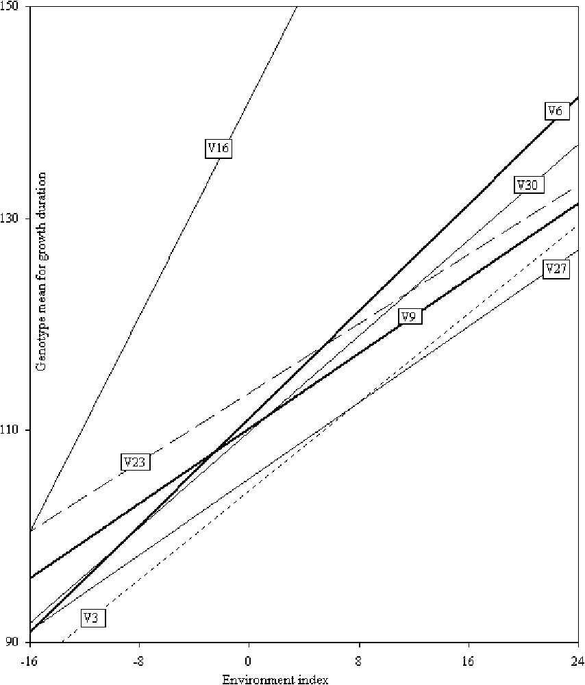
Linear regression showing the influence of different environments on the crop duration (days to flowering) of rice genotypes.

3.3 Measurement of interaction effects through AMMI model

The effect of genotype, environment and the components of $G \times E$ interactions were highly significant (Table 2). The environment SS was quite large. Also, the $G \times E$ interaction SS was about double as genotype SS. Most of the interaction SS was captured by the first IPCA axis. IPCA1 and IPCA2 together hold 97% of $G \times E$ SS. The root mean square (RMS) residuals were examined for model fit. The RMS residual for crop duration data in Table 2 was ${(1658 / 1920)}^{0.5} = 0.93$ day following AMMI4 model. Similarly, the RMS residual for AMMI2 was 1.26 days and that for AMMI1 was 2.06 days, or 1.90% of the grand mean (108.48 days). Table 3 listed the additive parameters (deviations) and the multiplicative effects (IPCA scores). The first four axes have been computed in the present analysis, although only first one or two are usually considered for interpretation. Expected crop duration (response) could be calculated from the table by using the AMMI model equation. For example, the AMMI1 expected crop duration for V1 grown in B1 would be $108.48 + (- 0.18) + (- 4.62) + [(- 0.11) \times (- 2.24)] = 103.93$ days. The observed duration was 106.67 days (Appendix I). Thus the AMMI1 model leaved a residual of 2.74 days. Moreover, V40 under H4 environment had leaved a residual of 6.94 days in AMMI1 model. It was estimated that AMMI1 model accounted for 97.7% of the observed data.

Genotypes/environments	Deviation (days)	IPCA score $(\sqrt{days})$
IPCA 1	IPCA 2	IPCA 3	IPCA 4
V1	−0.18	−0.11	−0.57	−0.15	−0.89
V2	−3.28	−0.38	−1.09	−0.17	−0.84
V3	−4.20	0.03	0.42	−1.18	0.58
V4	−10.26	0.14	2.60	−0.64	0.01
V5	−3.78	−0.54	−1.15	−0.23	−0.76
V6	2.64	0.99	−1.28	0.65	0.25
V7	−1.86	0.13	0.21	−0.40	0.04
V8	−12.32	−0.04	2.95	−0.76	−0.16
V9	1.72	−0.88	−0.64	−0.15	1.67
V10	−5.80	−0.19	1.42	−0.22	0.15
V11	−0.26	−0.15	−0.95	0.89	−1.23
V12	2.09	−1.08	−0.22	0.56	1.03
V13	2.53	−1.08	−0.19	0.72	0.68
V14	2.68	−1.05	0.27	0.39	0.28
V15	1.61	0.16	0.72	1.06	0.09
V16	57.68	17.26	−0.38	0.12	0.23
V17	−0.84	−0.87	−1.31	−0.51	−1.27
V18	−0.61	−0.51	−1.50	−0.12	−0.69
V19	−2.93	−0.25	1.24	2.46	−0.15
V20	−2.72	−0.40	−0.75	−0.50	−0.89
V21	−1.47	−0.68	−0.36	−0.35	0.18
V22	−1.11	−0.55	−0.33	−0.45	−0.19
V23	5.01	−1.30	−0.90	1.06	1.85
V24	−2.22	−0.53	−1.13	−0.27	0.12
V25	−2.80	−0.59	0.25	−1.43	0.53
V26	−3.14	−0.43	−0.45	−1.29	0.63
V27	−3.05	−0.53	2.02	−1.57	0.12
V28	2.01	−0.92	−1.34	−0.17	1.55
V29	−6.51	0.06	3.58	0.28	−0.20
V30	1.39	0.20	−1.97	−1.05	0.34
V31	−3.28	−0.25	−0.84	−1.15	−0.90
V32	−1.93	−0.81	0.02	−0.05	−0.50
V33	6.64	−0.99	−0.50	0.59	0.45
V34	2.14	−0.89	−0.86	−0.11	0.21
V35	−1.59	−0.38	−0.10	1.28	−0.36
V36	0.28	−0.81	−0.50	0.43	0.64
V37	−4.01	−0.10	2.62	−0.27	−0.17
V38	−5.16	−0.34	2.40	0.86	−0.42
V39	−0.14	−0.76	−0.43	1.99	−0.62
V40	−3.11	−0.55	−0.96	−0.13	−1.44

B1	−4.62	−2.24	−3.66	0.14	−0.60
B2	−17.50	−2.68	0.09	0.49	−0.41
B3	−16.60	−2.75	1.55	−0.30	0.01
B4	16.23	7.81	0.26	−0.55	−1.00
C1	−4.61	−2.46	−3.31	0.92	0.91
C2	−16.60	−2.74	0.26	−0.48	1.25
C3	−13.10	−2.64	2.25	−1.32	−0.70
C4	12.31	7.64	−0.14	0.26	0.72
D1	−2.14	−2.46	−3.38	0.85	−1.54
D2	−13.50	−2.63	0.56	−1.49	−2.78
D3	−11.00	−2.18	3.93	4.33	−0.31
D4	28.64	7.22	−0.28	0.23	0.32
H1	−4.71	−2.34	−2.04	0.07	2.15
H2	−16.60	−2.67	0.96	−1.14	0.30
H3	−15.40	−2.86	2.60	−1.81	1.65
H4	12.40	7.96	0.36	−0.19	0.03

Fig. 2 showed the expected crop duration considering mean duration on the abscissa and IPCA1 scores (for genotypes and environments) on the ordinate. Sixteen environments are shown with open circles. Filled tetragons denote the genotypes. The genotypes with similar positions were not shown in the graph. Eighteen genotypes out of 40 were presented in the AMMI biplot. Straight lines draw attention to the grand mean on the abscissa and to zero on the ordinate.

Fig. 2
AMMI1 model for crop duration (days to flowering) data, accounting for 97.7% of the treatment SS.

The genotypes V6, V8 and V37 showed more or less similar distances from the horizontal reference line. However, series of displacements along the abscissa indicated their differences due to only main effects. On the other hand, V6, V9, V15, V28 and V30 are being dispersed along the ordinate and apparently they differ only in interaction effects. The genotypes V8 and V28 differ in both; while V1, V10, V20, V27 and V38 are rather similar with respect to both main effects and interaction effects.

The main effect for genotypes reflects breeding advances and the main effect for environments characterize the site [21]. Considering these responses, the four environments viz. B4, C4, D4 and H4 had exhibited remarkably longer life span of rice plants (Table 3 and Fig. 3). On the other hand, environments B2, C2, H2, B3 and C3 were characterized by extremely short duration. In general, shorter duration of rice varieties produces inferior yield mainly because of lower amount of solar radiation received.

Fig. 3
AMMI2 model for the interaction of crop duration (days to flowering) data.

Direction and level of interactions of genotypes with environments could be determined from Fig. 2. For example, V16 had strong positive interactions with the environments B4, C4, D4 and H4, and strong negative interactions with all other 12 environments. In fact, this variety could not emerge panicle at all in the Boro season in all four locations. As a result, its duration was extended up to the next T. Aman crop. On the other hand, V9, V28 and V33 had strong positive interactions with D3, little interactions with B1 and H1, and strong negative interactions with B4, C4, D4 and H4. In general, local aromatic rice varieties possess photoperiod sensitivity at varying degrees. For this reason, life span might be flexible depending on planting time and season. Negative interaction for duration may be preferred up to a certain limit of grain yield reduction.

For further observation of interaction effects exclusively, a different type of biplot had been presented in Fig. 3. It held IPCA1 on the abscissa and IPCA2 on the ordinate. It captured 97% of the interaction as against 92% of Fig. 3. Figs. 2 and 3 together effectively captured 99% of the treatment SS in the AMMI2 model, leaving a RMS residual of only 1.26 day, or 1.16% of the grand mean (Table 2). Principles of biplot graph for IPCA1 and IPCA2 were described by Kempton where he proved efficiency of this type of graph in the explanation of interactions [26]. The genotypes V1, V3, V7, V9, V15, V20 and V33 and the environments B2, C2 and D2 are situated very near the origin. It indicated a little interaction for the entities (varieties and environments). Therefore the genotypes V1, V3, V7, V9, V15, V20 and V33 are stable over the environments and the environments B2, C2 and D2 are more stable environments for all the rice genotypes.

Note

References

[1] O.H. Frankel The IRRI phytotron: Science in the service of human welfare (Anonymous, ed.), Proceedings of the Symposium on Climate & Rice, Int. Rice Res. Inst., Los Baños, Laguna, Philippines, 1976, pp. 3-9

[2] R. Knight The measurement and interpretation of genotype–environment interactions, Euphytica, Volume 19 (1970), pp. 225-235

[3] M. Murugesan; K.P. Dhamu; R.A. Arokia Genetic variability in some quantitative characters of sesame, Madras Agric. J., Volume 66 (1979), pp. 366-369

[4] M.S. Swaminathan Rice in 2000 AD (Y.P. Abrol; Sulochana Gadgil, eds.), Rice – In a Variable Climate, APC Publications Pvt. Ltd., New Delhi, India, 1999, pp. 217-238

[5] C. Chu; P.S. Tang Studies on plant respiration. IV. Some morphological, physiological and biochemical changes during germination of rice at different partial pressures of oxygen, Acta Bot. Sin., Volume 8 (1959), pp. 201-214

[6] K.W. Finlay; G.N. Wilkinson The analysis of adaptation in plant breeding programme, Aust. J. Agric. Res., Volume 14 (1963), pp. 742-754

[7] T.T. Chang; B.S. Vergara Ecological and genetic information on adaptability and yielding ability in tropical rice varieties (Anonymous, ed.), Rice Breeding, Int. Rice Res. Inst., Los Baños, Laguna, Philippines, 1972, pp. 431-453

[8] S. Yoshida Fundamentals of Rice Crop Science, Int. Rice Res. Inst., Los Baños, Laguna, Philippines, 1981

[9] D.K. Bagchi; P. Banik; T. Sasma Selection of appropriate technologies for upland rice growing on the Bihar plateau, India (Anonymous, ed.), Fragile Lives in Fragile Ecosystems, Int. Rice Res. Inst., Los Baños, Philippines, 1995, pp. 127-134

[10] M. Dingkuhn; A. Sow; A. Samb; S. Diack; F. Asch Climatic determinants of irrigated rice performance in the Sahel. I. Photothermal and micro-climatic responses of flowering, Agric. Syst., Volume 48 (1995), pp. 385-410

[11] M. Dingkuhn; K.M. Miezan Climatic determinants of irrigated rice performance in the Sahel. II. Validation of photothermal constants and characterization, photothermal of genotypes, Agric. Syst., Volume 48 (1995), pp. 411-433

[12] M. Dingkuhn; F. Asch Phenological responses of Oryza sativa, O. glaberrima and inter-specific rice cultivars on a toposequence in West Africa, Euphytica, Volume 110 (1999), pp. 109-126

[13] B.S. Vergara; T.T. Chang The Flowering Response of the Rice Plant to Photoperiod: A Review of the Literature, Int. Rice Res. Inst., Los Baños, Laguna, Philippines, 1985

[14] R.K. Singh; U.S. Singh; G.S. Khush Aromatic Rices, Oxford and IBH Publishing Co. Pvt. Ltd., New Delhi, 2000

[15] Anonymous, Bangladesh Rice Research Institute: Serving the Nation, BRRI publication no. 119, Bangladesh Rice Res. Inst., Gazipur 1701, Bangladesh, 1997

[16] A. Hamid, N. Uddin, M. Haque, E. Haque, Deshi dhaner jat, BRRI publication no. 59, Bangladesh Rice Res. Inst., Gazipur 1701, Bangladesh, 1982

[17] N.M. Miah, H.C. Sarkar, Evaluation of semidwarf rice mutants in Bangladesh, BRRI publication no. 96, Bangladesh Rice Res. Inst., Gazipur 1701, Bangladesh, 1990

[18] J.K. Ladha; G.J.D. Kirk; J. Bennett; S. Peng; C.K. Reddy; P.M. Reddy; U. Singh Opportunities for increased nitrogen use efficiency from improved lowland rice germplasm, Field Crops Res., Volume 56 (1998), pp. 41-71

[19] S.A. Eberhart; W.L. Russel Stability parameters for comparing varieties, Crop Sci., Volume 6 (1966), pp. 34-40

[20] J. Ram; O.P. Jain; B.R. Murty Stability performance of some varieties and hybrid derivatives in rice under high yielding varieties programme, Indian J. Genet. Plant Breed., Volume 30 (1970), pp. 187-198

[21] R.W. Zobel; M.W. Wright; H.G. Gauch Statistical analysis of a yield trial, Agron. J., Volume 80 (1988), pp. 388-393

[22] Q.A. Haque; N.M. Miah; M.A. Kabir; P.K.S. Ray; M.U. Ghani; M.L. Ali; M.S. Islam Yield stability of some rice genotypes in South Asia, Bangladesh Rice J., Volume 2 (1991), pp. 69-74

[23] S.K. Sinha; S. Biswas Adaptability of some rice varieties in unilocational testing programme during aus season, Oryza, Volume 23 (1986), pp. 166-172

[24] R.K. Das; M.K. Bashar; N.M. Miah; M. Nasiruddin Genotype–location interaction in upland rice, Bangladesh J. Plant Breed. Genet., Volume 4 (1991), pp. 15-20

[25] D. Mishra; S.K. Dash Genetic diversity and stability in aromatic rice (Oryza sativa L.), Indian J. Agric. Sci., Volume 67 (1997), pp. 27-29

[26] R.A. Kempton The use of biplots in interpreting variety by environment interactions, J. Agric. Sci. Camb., Volume 103 (1984), pp. 123-135

Comments - Policy