

1 Introduction
Since the pioneering work of Volterra [1] and Lotka [2] in the mid-1920s, there has been increasing interest in investigating the dynamical behaviors of predator–prey models in both ecology and mathematical ecology [3–11]. In particular, one of the important dynamical predator–prey behaviors, such as periodic phenomena and bifurcation has become even more interesting [6–10,12–24]. In 1980, Freeman [25] proposed a most popular predator–prey model with Michaelis–Menten-type functional response:
| (1) |
Considering that in many situations, predators must search and share or compete for food, Arditi and Ginzburg [3] introduced and studied the following ratio-dependent-type functional response model:
| (1.2) |
Since the functional response depends on the predator density in a different way, Hassel and Varley [26] reconstructed the predator–prey model with Hassell–Varly-type functional response, which takes the following form:
| (1.3) |
| (1.4) |
| (1.5) |
| (1.6) |
In this paper, we will devote our attention to investigating the properties of a Hopf bifurcation of system (1.6), that is to say, we shall take the delay τ as the bifurcation parameter and show that when τ passes through a certain critical value, the positive equilibrium loses its stability and a Hopf bifurcation will take place. Furthermore, when the delay τ takes a sequence of critical values containing the above critical value, the positive equilibrium of system (1.6) will undergo a Hopf bifurcation. In particular, by using the normal form theory and the center manifold reduction due to Faria and Maglhalaes [28], the formulae for determining the direction of Hopf bifurcations and the stability of bifurcating periodic solutions are obtained. In addition, the existence of periodic solutions for τ far away from the Hopf bifurcation values is also established by means of the global Hopf bifurcation result of Wu [29].
In order to obtain the main results of our paper, throughout this paper, we assume that the coefficients of system (1.6) satisfy the following condition: am2 + cd − cr > 0, r > dH1
This paper is organized as follows. In Section 2, the stability of the positive equilibrium and the existence of a Hopf bifurcation at the positive equilibrium are studied. In Section 3, the direction of Hopf bifurcation and the stability of bifurcating periodic solutions on the center manifold are determined. In Section 4, numerical simulations are carried out to illustrate the validity of the main results. In Section 5, some conditions that guarantee the global existence of the bifurcating periodic solutions to the model are given. Biological explanations and some main conclusions are drawn in Section 6.
2 Stability of the equilibrium and existence of the local Hopf bifurcation
In the section, by analyzing the characteristic equation of the linearized system of system (1.6) at the positive equilibrium, we investigate the stability of the positive equilibrium and the existence of the local Hopf bifurcations occurring at the positive equilibrium.
Considering the biological meaning, we only study the property of a unique positive equilibrium (i.e., coexistence equilibrium). It is easy to see that under the hypothesis (H1), system (1.6) has a unique positive equilibrium , where
Let then, system (1.6) takes the following form:
| (2.1) |
Then, we obtain the linearized system of (2.1)
| (2.2) |
| (2.3) |
In order to investigate the distribution of roots of the transcendental equation (2.3), the following Lemma stated in [30] is helpful.
Lemma 2.1.[30]For the transcendental equation
Regarding τ as the parameter, we can apply Lemma 2.1 to (2.3), which is a special case of
Obviously, if m1n2 ≠ m2n1, then, λ = 0 is not a root of (2.3). For τ = 0 the characteristic equation (2.3) becomes:
| (2.4) |
It is easy to see that Eq. (2.4) have two negative real roots if the following condition: m1 + n2 < 0, m1n2 − m2n1 > 0H2
Multiplying eλτ on both sides of (2.3), it is obvious to obtain:
| (2.5) |
For ω0 > 0, iω0 is a root of (2.5) if and only if
| (2.6) |
Separating the real and imaginary parts of (2.6), we get:
| (2.7) |
If the condition (H2) holds, we can easily check that cosω0τ ≠ 0. Then, it follows from (2.7) that:
| (2.8) |
From the second equation of (2.7), we can easily obtain:
| (2.9) |
From (2.7), we know that (2.3) has a simple pair of purely imaginary roots ±iω0 at
Let be the root of Eq. (2.3) satisfying
Assume thatH3
Then, the following transversality condition holds.
Proof. Differentiating the equation (2.3) with respect to τ leads to:
When τ = τk, iω0 is a purely imaginary root of (2.3). We then easily get:
| (2.10) |
From (2.7), we have:
Hence,
Under the condition (H3), we know that
Applying Lemma 2.1, we obtain the following results: Lemma 2.3. If (H1), (H2) and (H3) are satisfied, then
(i) if , all roots Eq. (2.3) have negative real parts;
(ii) if τ = τ0, all roots of Eq. (2.3) except ±iω0 have negative real parts;
(iii) if τ ∈ [τk, τk+1) for k = 0, 1, 2, ..., Eq. (2.3) have 2 (k + 1) roots with positive real parts.
Spectral properties of Eq. (2.3) immediately lead to the properties of the zero solutions to system (2.2), and equivalently, of the positive equilibrium E∗ for system (1.6).
Theorem 2.4.Suppose that (H1), (H2) and (H3) are satisfied. Then, the positive equilibrium E∗of system(1.6)is asymptotically stable when, and unstable when τ > τ0. Moreover, at τ = τk, k = 0, 1, 2, ..., ± iω0 are a simple pair imaginary roots of (2.3), and (1.6) undergoes a Hopf bifurcation near E∗.
3 Direction and stability of the Hopf bifurcation
In the previous section, we have obtained conditions for Hopf bifurcations to occur when τ = τk. In this section, we will employ the algorithm of Faria and Maglhalaes [28] to compute explicitly the normal forms of system (1.6) on the center manifold. After that, we will investigate the direction of the Hopf bifurcation and stability of the bifurcating periodic orbits from the positive equilibrium E∗ of system (1.6) at these critical values of τk. We know that Eq. (2.3) has a pair of purely imaginary roots ±iω0 when τ = τk and system (1.6) undergoes a Hopf bifurcation from E∗. Let μ = τ–τk, then μ = 0 is the Hopf bifurcation value of system (1.6).
Throughout this section, we refer to Faria and Maglhalaes [28] for the meaning of the notations involved.
Normalizing the delay τ by the time-scaling t → t/τ, then the system (2.1) can be rewritten as a functional differential equation in :
| (3.1) |
Let u = (u1(t), u2(t))T, then, system (3.1) can be rewritten in the following vector form:
| (3.2) |
Obviously, L(τ) is a continuous linear function mapping into R2. By the Riesz representation theorem, there exists a 2 × 2 matrix function , whose elements are of bounded variation such that
| (3.3) |
In fact, we can choose
| (3.4) |
| (3.5) |
From Lemma 7.1.1 in Hale [32], we know that , is a strongly continuous semigroup of linear transformation on and the infinitesimal generator A(τ) of T(t), t ≥ 0 is given by
| (3.6) |
| (3.7) |
For , define
| (3.8) |
| (3.9) |
Consider the complex coordinates and still denote as C. Suppose that Φ = (Φ1, Φ2) is a basis of P and
Also, the two eigenvectors Ψ1, Ψ2 of A* corresponding to the eigenvalues iω0τk, –iω0τk, respectively, construct a basis Ψ = (Ψ1, Ψ2)T of the adjoint space P* of P and
Thus, where I2 is a second-order identical matrix. It is known that , where
Take the enlarged phase space C by considering the space The projection of C upon P, associated with the decomposition C = P⊕Q, is now replaced by π : BC → P such that .
Thus, we have the decomposition BC = P⊕Kerπ. Using the decomposition , and by Theorem 7.6.1 in [32], we can decompose (3.2) as
| (3.10) |
| (3.11) |
| (3.12) |
In what follows, we first define the operators as
| (3.13) |
In particular, is the canonical basis for C2. Therefore, we have
By (3.10), we have
| (3.14) |
Noting that L(μ) = μ / τkL(τk), we have
| (3.15) |
| (3.16) |
Since the second-order terms in (μ, x) on the center manifold are given by
| (3.17) |
| (3.18) |
In the following, we shall compute the cubic term . First, we note that
However, the terms are irrelevant to determine the generic Hopf bifurcation. Hence, it is only needed to compute the coefficients of and . Let
From (3.1) and (3.2) and from (3.18) we can easily see that and
Therefore, we have . In the sequel, we only need to compute and h(x)(θ).
From (3.15), we have:
In view of the definition of , the equation can be written as the following partial differential equations:
| (3.19) |
From (3.19), we can easily obtain:
Thus, we obtain:
In what follows, we shall compute . From (3.14), we know
| (3.20) |
| (3.21) |
Thus, from (3.20), we obtain
Therefore,
Since h110(θ) and h200(θ) for appear in B3, we still need to compute them.
Following [28], we know that h = h (θ; x1, x2, μ) is the unique solution in the linear space of homogeneous polynomials of degree 2 in 3 real variable (x, μ) = (x1, x2, μ) of the equation
| (3.22) |
| (3.23) |
Combining the definition (3.6) of the operator A(τ), we can obtain:
For the sake of simplicity, let:
| (3.24) |
Then, h0 can be evaluated by the system
| (3.25) |
| (3.26) |
In view of (3.14), (3.15), (3.25) and (3.26), we know that and are the solution to the following two equations:
| (3.27) |
| (3.28) |
Solving the Eq. (3.27) and (3.28), we have
| (3.29) |
| (3.30) |
| (3.31) |
| (3.32) |
| (3.33) |
Accordingly, the normal form (3.12) of (3.10) has the following form
The normal form (3.12) relative to P can be written in real coordinates (ω1, ω2) through the change of variables x1 = ω1 − iω2, x2 = ω1 + iω2. Setting ω1 = ρ cosν, ω2 = ρ sinν, then this form becomes
| (3.34) |
Summarizing the above analysis, we have the following result.
Theorem 3.1.The flow of Eq.(3.2)with μ = 0 on the center manifold of the origin is given by (3.34). Hopf bifurcation is supercritical if k1k2 < 0 and subcritical if k1k2 > 0. Moreover, the nontrivial periodic solution is stable if k2 < 0 and unstable if k2 > 0.
4 Numerical examples
In this section, we present some numerical results for some particular values of the parameters associated with the model system (1.6). We consider the system (1.6) with a = 1, b = 2, c = 0.3, m = 0.5, d = 0.8, r = 2. That is,
| (4.35) |
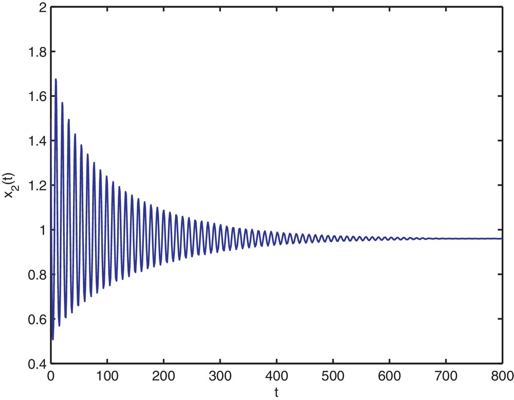
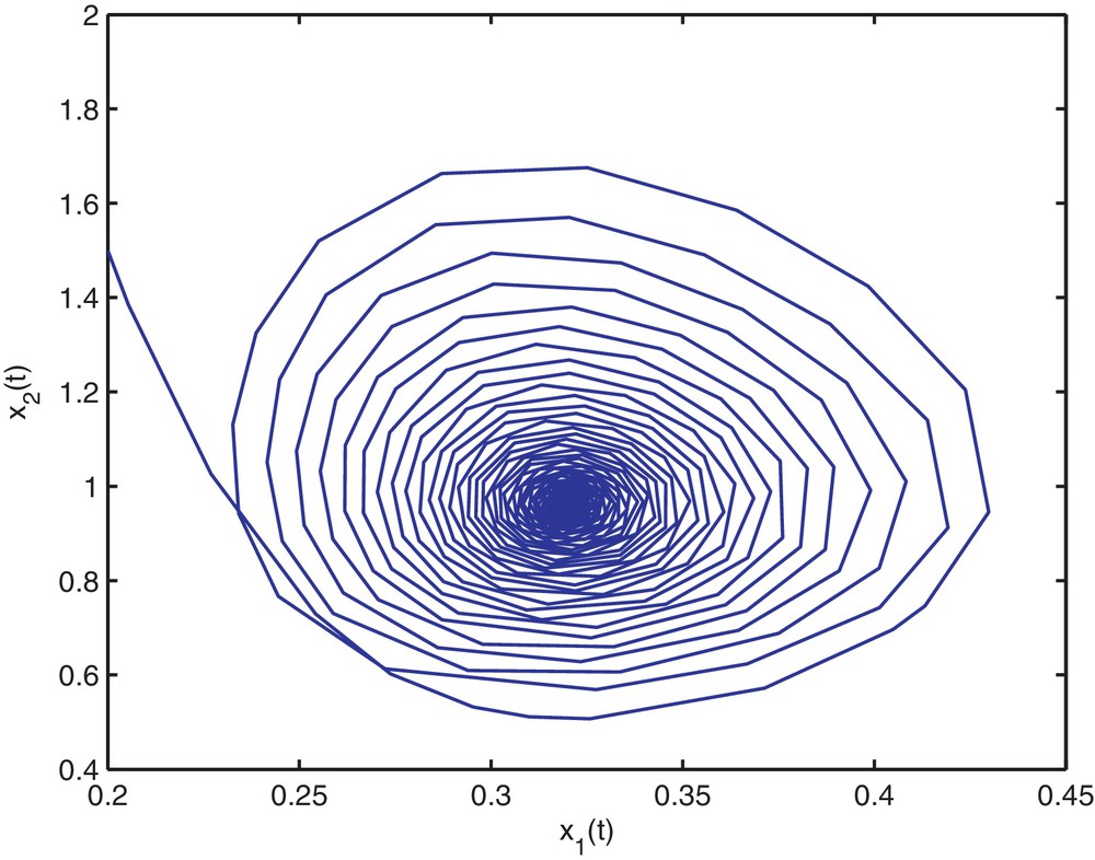
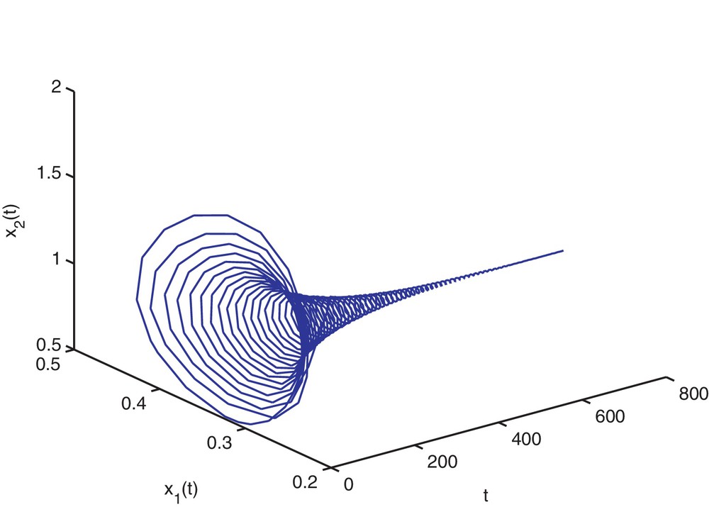
Then, the stability determining quantities for Hopf bifurcating periodic solutions are given by k1 = 0.1912, k2 = −0.1377. From Theorem 2.4, we know that the positive equilibrium is asymptotically stable when and is unstable when τ > 1.94. The numerical simulations for τ = 1.9 and τ = 2 are shown on Figs. 1–8, respectively. From Theorem 3.1, we know that system (4.35) with τ = 1.94 has a supercritical Hopf bifurcation and the nontrivial periodic solution bifurcating from the Hopf bifurcation of (4.35) with τ = 1.94 is orbitally asymptotically stable on the center. Moreover, all the roots of Eq. (2.3) with τ = 1.94, except ±0.9254i, have negative real parts. Thus, the center manifold theory implies that the stability of the periodic solutions projected on the center manifold coincides with the stability of the periodic solutions in the whole phase space.
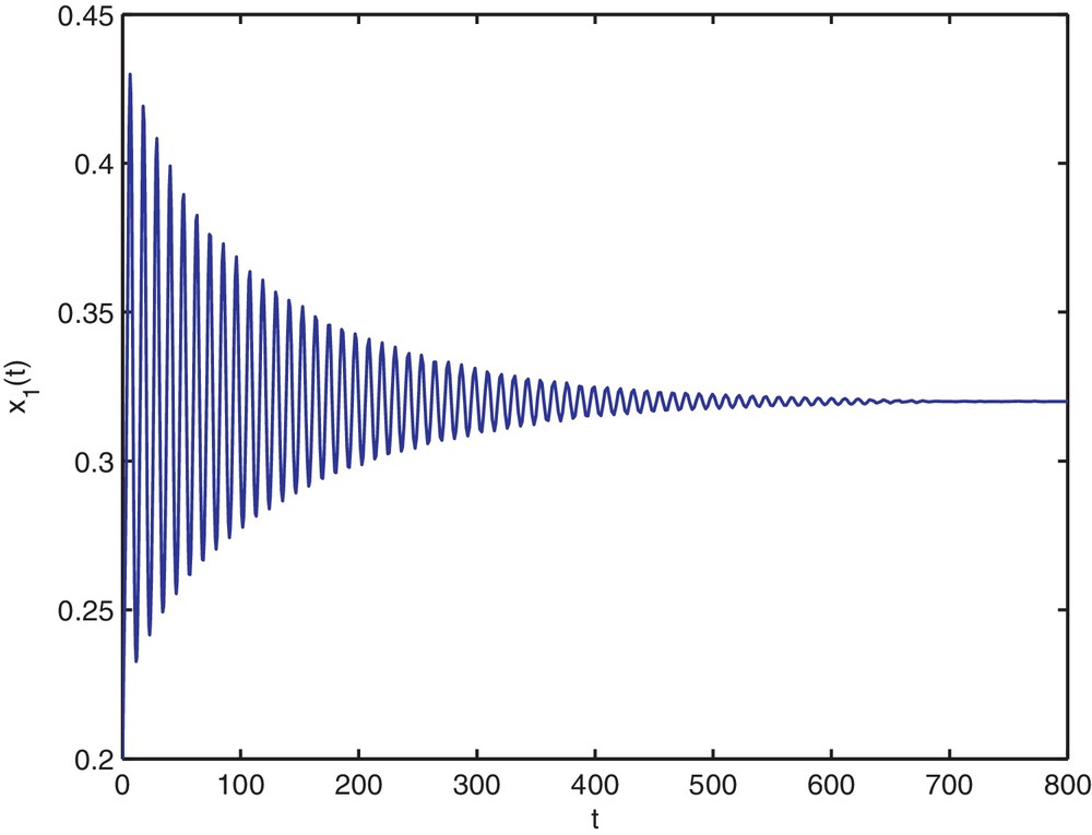
Trajectory portrait and phase portrait of system (4.35) with τ = 1.9 < τ0 ≈ 1.94. The positive equilibrium is asymptotically stable. The initial value is (0.2, 1.5).
Trajectory portrait and phase portrait of system (4.35) with τ = 1.9 < τ0 ≈ 1.94. The positive equilibrium is asymptotically stable. The initial value is (0.2, 1.5).
Trajectory portrait and phase portrait of system (4.35) with τ = 1.9 < τ0 ≈ 1.94. The positive equilibrium is asymptotically stable. The initial value is (0.2, 1.5).
Trajectory portrait and phase portrait of system (4.35) with τ = 1.9 < τ0 ≈ 1.94. The positive equilibrium is asymptotically stable. The initial value is (0.2, 1.5).
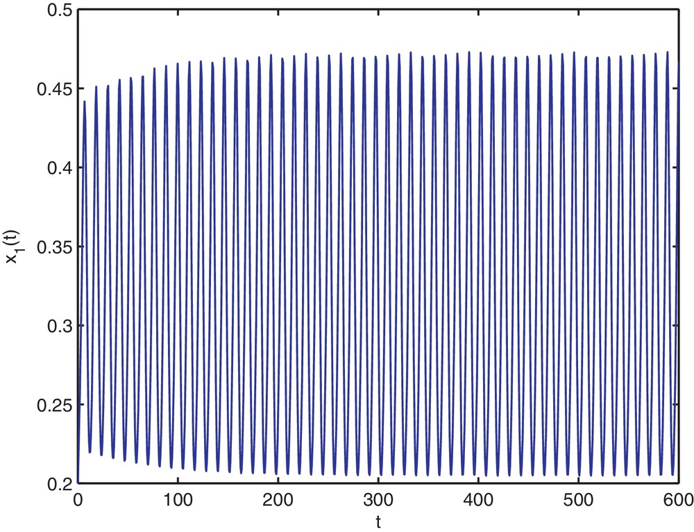
Trajectory portrait and phase portrait of system (4.35) with τ = 2 < τ0 ≈ 1.94. Hopf bifurcation occurs from the positive equilibrium . The initial value is (0.2, 1.5).
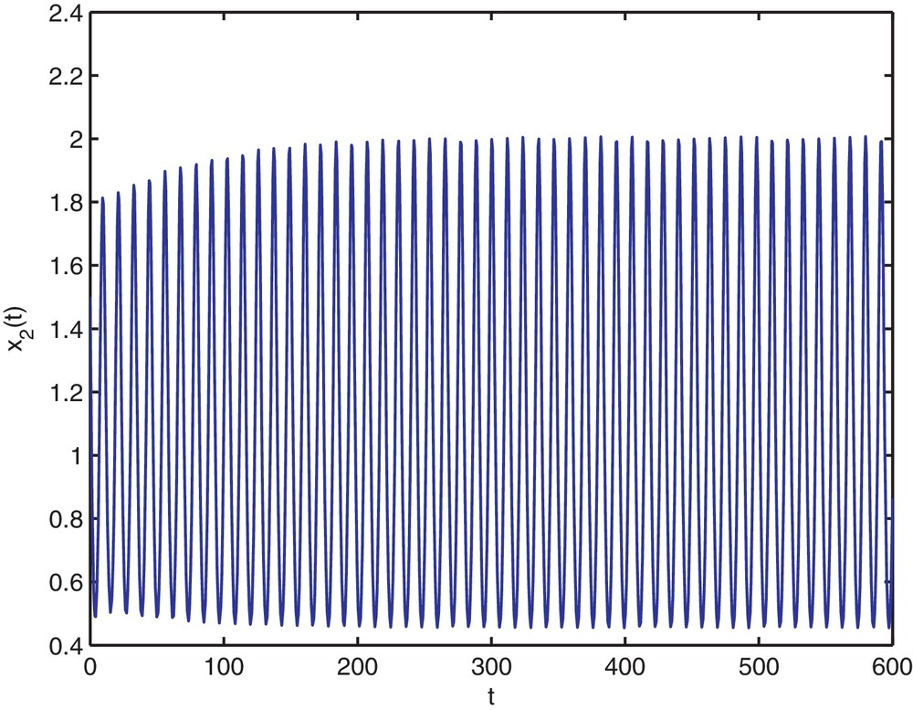
Trajectory portrait and phase portrait of system (4.35) with τ = 2 < τ0 ≈ 1.94. Hopf bifurcation occurs from the positive equilibrium . The initial value is (0.2, 1.5).
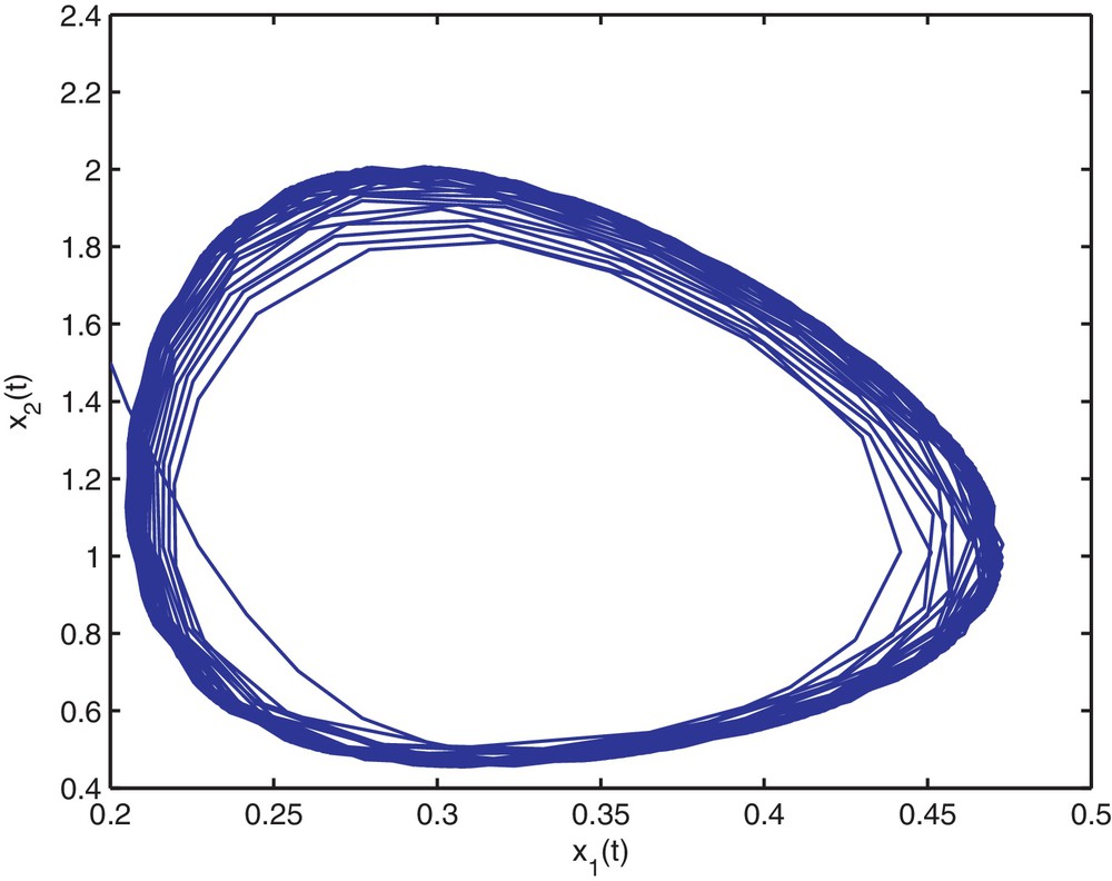
Trajectory portrait and phase portrait of system (4.35) with τ = 2 < τ0 ≈ 1.94. Hopf bifurcation occurs from the positive equilibrium . The initial value is (0.2, 1.5).
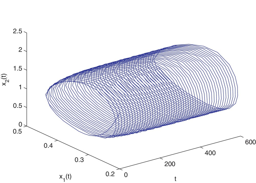
Trajectory portrait and phase portrait of system (4.35) with τ = 2 < τ0 ≈ 1.94. Hopf bifurcation occurs from the positive equilibrium . The initial value is (0.2, 1.5).
5 Global continuation of local Hopf bifurcations
In the earlier sections we have established that the model system (1.6) undergoes a Hopf bifurcation at for τ = τk and also investigated the stability of bifurcating periodic solutions. We all know that periodic solutions can arise through the Hopf bifurcation in delay differential equations. However, these bifurcating periodic solutions are generally local, i.e., they only exist in a small neighborhood of the critical value. Therefore, we want to know that whether these nonconstant periodic solutions obtained through local Hopf bifurcations exist globally or not. In this section, we will consider the global continuation of periodic solutions bifurcating from the positive equilibrium of system (1.6).
Throughout this section, we closely follow the notations in Wu [29]. For the simplification of notations, setting , we can rewrite system (1.6) as the following form
| (5.1) |
Following the work of Wu [29], we need to define:
Let be the equilibrium of system (5.1). Then, the characteristic matrix of (5.1) at the equilibrium takes the following form
For the benefit of the readers, we first state the global Hopf bifurcation theory due to Wu [29] for functional differential equations.
Lemma 5.1. Assume that is an isolated center satisfying the hypotheses (A 1 ) – (A 4 ) in Wu [7] . Denote by
the connected component of in Γ. Then, either
(i) is unbounded, or
(ii)is bounded, is finite and
Obviously, if (ii) of Lemma 5.1 is not true, then is unbounded. Thus, if the projections of onto z-space and onto p-space are bounded, then the projections of onto τ-space is unbounded. Further, if we can show that the projections of onto τ-space is away from zero, then the projections of onto τ-space must include the interval . Based on the idea, we can prove our results on the global continuation of the local Hopf bifurcation.
Lemma 5.2. If τ is bounded, then all periodic solutions to (1.6) is uniformly bounded.
Proof. Let be a nontrivial solution to (1.6) and define
Thus, which implies that solutions to (1.6) cannot cross the x-axes and y-axes. Thus, the nonconstant periodic orbits must be located in the interior of the first quadrant. If (x1(t), x2(t)) is a solution to (1.6), then it follows from the first equation of (1.6) that
| (5.2) |
Clearly, for t > τ, which implies that . This, together with (5.2), leads to
Thus,
From the second equation of (1.6), we have
Then,
Therefore,
Applying the second equation of (1.6), we get
i.e.
It follows that
Thus, the possible periodic solutions lying in the first quadrant of (1.6) must be uniformly bounded. This completes the proof of Lemma 5.2.
Lemma 5.3.If a < d, r < c, then system (1.6) has nonconstant periodic solution with period τ.
Proof. Suppose for a contradiction that system (1.6) has a nonconstant periodic solution with period τ. Then, the following ordinary differential equations
| (5.3) |
Note that x-axis and y-axis are the invariable manifold of system (5.3) and the orbits of system (5.3) do not intersect each other. Thus, there are no solutions crossing the coordinate axes. On the other hand, consider that if system (5.3) has a periodic solution, then there must be an equilibrium in its interior, and that E0(0, 0) is located on the coordinate axis. Thus, we can conclude that the periodic orbit of system (5.3) must lie in the first quadrant.
In the sequel, we will prove that system (5.3) has no nonconstant periodic solution in the first quadrant.
Define
It is easy to show that D is an ultimately bounded region (or absorbing and positively invariant set) of system (5.3). Let
Then, a direct computation show that, for (x, y) ∈ D and a < d, r < c,
Thus, the Bendixson–Dulac criterion, together with the fact that D is an ultimately bounded region of (5.3), implies that (5.3) has no nontrivial periodic solutions, leading to a contradiction. Thus, the proof is complete.
Theorem 5.4.Assume that a < d, r < c. Let ω0 and τk (k = 0,1,2,…) be defined by (2.8) and (2.9), respectively. Then, for each τ > τk (k ≥ 1), system (1.6) has at least k periodic solutions.
Proof. Obviously, is an isolated center of (1.6). Let
denote the connected component passing through in Γ. It follows from Theorem 2.4 that is nonempty. It is only necessary to prove that the projection of onto τ-space is for each j > 0, where .
By Lemma 2.2 and 2.3, there exists ɛ > 0, δ > 0 and a smooth curve λ: (τk – δ, τk + δ) → C such that for all , and
Let . It is easy to verify that on , if and only if μ = 0, τ = τk and . This verifies assumption (A4) of Wu [29]. Moreover, if we put
By Theorem 3.3 of Wu [29], we conclude that the connected component through in Σ is nonempty, and
Thus, is unbounded. From (2.9), one can show that, for k ≥ 1,
Hence,
| (5.4) |
Now, we are in position to prove that the projection of onto τ-space is [τ, ∞), where τ ≤ τk. Clearly, It follows from the proof of Lemma 5.3 that system (1.6) with τ = 0 has no nontrivial periodic solution. Hence, the projection of onto τ-space is away from zero.
For the sake of contradiction, we suppose that the projection of onto τ-space is bounded. This means that the projection of onto τ-space is included in an interval (0, τ*). From (5.4) and applying Lemma 5.3, we get 0 < p < τ* for . This implies that the projection of onto p-space is also bounded. Thus, combining this with Lemma 5.2, we can get that the connected component is bounded. This contradiction completes the proof.
6 Conclusions and biological explanations
In this paper, we have investigated the local stability of the positive equilibrium and the local Hopf bifurcation in a delayed predator–prey model with Hassell–Varley-type functional response. We have showed that if conditions (H1)–(H3) hold, the positive equilibrium of system (1.6) is asymptotically stable for all τ ∈ [0, τ0) and unstable for τ > τ0. This shows that, in this case, the population of preys and predators will tend to stabilization and still keep stable whenever the delay parameter lies in the range τ ∈ [0, τ0) and unstable when τ > τ0. We have also showed that, if conditions (H1)–(H3) hold, as the delay τ increases, the equilibrium loses its stability and a sequence of Hopf bifurcations occur at , i.e., a family of periodic orbits bifurcate from the positive equilibrium . This means that the population of preys and predators may coexist and keep in an oscillatory mode. Moreover, the direction of Hopf bifurcation and the stability of the bifurcating periodic orbits are discussed by applying the normal form theory and the center manifold theorem. Numerical simulations supporting our theoretical results are also included. Further, sufficient conditions ensuring the existence of global Hopf bifurcation are given, i.e., if a < d, r < c, then system (1.6) has at least k periodic solutions for τ > τk(k ≥ 1). It is shown that the population of preys and predators still keep in an oscillatory mode near the positive equilibrium for τ > τk(k ≥ 1).