1 Introduction
In recent years, there has been an increasing interest to develop new state and parameter estimation schemes to reduce the deficiencies of classical schemes such as the Kalman Filter (KF) and the Luenberger Observer (LO) which have been frequently used to reconstruct variables that are not measured and to reduce the effect of noise on the available measurements. However, due to the fact that the stability and convergence properties of these estimators are essentially locally valid, their application has been restrictive in many practical situations. Other estimation approaches (the high gain [1], adaptive [2], and sliding mode [3]) have been also devised to solve the state reconstruction problem since the stability of the system is guaranteed but their designs involve conditions that must be assumed a priori or that are usually hard to verify [4]. These may account for the failure of these estimators to find widespread application in biological processes [2].
In this paper we present an innovative state estimation schemes to overcome the difficulties associated with the reconstruction of important nonmeasured variables in biological processes. It is based on the well-known Asymptotic Observer (AO) [2], which has proved to be suitable for certain biological processes by yielding satisfactory estimates in the face of uncertain kinetic parameters and load disturbances despite the dependence of the AO performance and convergence on the system operating conditions (particularly on the dilution rate which may be relatively low in most industrial scale biological processes) that have prevented the implementation of efficient monitoring and control strategies.
The objective of this study is then to propose an alternative to tune the convergence rate of a typical AO to compensate the effect of this plant features dependence of asymptotic observers by reducing the close interaction of the plant parameters in the estimator equations. This is accomplished by adopting a methodology similar to that used in [5] for a single-dimension bounded error observer, which is further developed to more complex n-dimensional cases. The main result is the inclusion of an adjustable convergence rate in the design of asymptotic observers while maintaining the stability and robustness convergence properties in the presence of nonlinear terms (i.e., process kinetics) and under the influence of load disturbances. The performance improvement of the classical asymptotic observer is finally demonstrated by applying in simulations the proposed tunable observer in an anaerobic digestion wastewater treatment process.
2 The considered general model
Let us consider the general class of biological systems that fits within the following model [2]:
| (1) |
| (2) |
- (H1) The matrix is known and bounded , i.e., there exist constant matrices and such that .
- (H2) The matrix C is constant and known with the property .
- (H3) The vector is known .
The operator ⩽ applied between vectors and between matrices should be understood as a collection of inequalities between elements.Note
3 A robust asymptotic observer
Under hypotheses (H1) to (H3), the following system designed by the linear transformation :
| (3) |
| (4) |
- (H4) .
- (H5) and are Hurwitz stable.
The hypothesis (H4) simply states that the matrix and thus, the matrices and are cooperative [7], while the hypothesis (H5) states the stability of these two constant matrices.
Under hypotheses (H1)–(H5) the asymptotic observer (3) is stable and converges asymptotically towards for any set of initial conditions.Lemma 1
The proof of this lemma is given in [8].
4 A robust tunable asymptotic observer
This section presents the main results of this study. The most important limitation of observer (3) is indeed that, in most of the cases, its convergence rate is fixed by the operating conditions of the biological system (namely the dilution rate). To face this limitation, a change in the observer design is introduced in the following in order to obtain adjustable convergence rates.
Let us consider the following modified transformationwithand where, the gain matrix, is a continuously derivable function matrix with the property: Proposition
Then, under hypotheses (H1) to (H5), the following dynamical system (5)
where (6)
is a stable tuning asymptotic observer for model (1).(7)
Let be the observation error associated to (6). Under hypotheses (H1) to (H3), it is straightforward to verify that the error dynamics is given by Proof
Convergence and stability
with (8)
Now, since , it is clear that:
- (i) ,
- (ii) , and thus,
- (iii) .
Clearly, the advantage of the tunable observer (6) over the classical AO is that, by choosing a suitable gain matrix , the classical AO is provided with an adjustable convergence rate, which can be tuned by the user. Notice that influences both the stability and the convergence properties (see Eq. (8)) of the tuning observer and it can be properly chosen to accelerate the convergence rate which allows to reach the zero steady state, , even if the uncertainty of the nonlinear terms is reasonable high. It is also worth mentioning that, with the exception of the property (5), no other restrictions are imposed on the gain matrix . Thus, the choice of , may be, at a first glance, a relatively easy task. In other words, must be chosen to give the fastest convergence to the true state. Moreover, one can see that, as , the knowledge of the nonlinearities is no longer required and therefore, the tuning observer design converges to the classical AO with the same robustness, stability and convergence properties of the AO. Furthermore, if is chosen as , with , a fully decoupled tuning observer is obtained, where the parameters needed to tune each estimated state variable, , are exclusively those involved in the function . In the following section the proposed tuning observer will be applied to an actual highly nonlinear biological wastewater treatment process.
5 Application to wastewater treatment processes
Anaerobic Digestion (AD) is a series of multi-substrate multi-organism biological processes that take place in the absence of oxygen and by which organic matter (expressed as COD, the Chemical Oxygen Demand) is decomposed and converted into biogas, a mixture of mainly carbon dioxide and methane, microbial biomass and residual organic matter [9]. Several advantages are recognised to AD processes when used in wastewater treatment processes: high capacity to treat slowly degradable substrates at high concentrations, very low sludge production, potentiality for production of valuable intermediate metabolites, low energy requirements and possibility for energy recovery through methane combustion. AD is indeed one of the most promising options for delivery of alternative renewable energy carriers, such as hydrogen, through conversion of methane, direct production of hydrogen, or conversion of by-product streams. However, despite these large interests and few thousands commercial installations refereed world-wide [10], many industries are still reluctant to use AD processes, probably because of the counterpart of their efficiency: they can become unstable under some circumstances. Hence, actual research aims not only to extend the potentialities of anaerobic digestion [11], but also to optimise AD processes and increase their robustness towards disturbances [12]. The design of efficient state estimators clearly goes in these two last directions since instrumentation is usually scarce at industrial scale.
5.1 An anaerobic digestion model
Let us consider the following dynamical model (known as AM1) for continuous anaerobic digestion process [13]. This model is given in the following matrix form (see Fig. 1) or simply which matches exactly model (1) with . In (9), the dotted lines indicate the partitions of Eq. (2). In this model, , , , and , are the concentrations of acidogenic bacteria, methanogenic bacteria, COD, Volatile Fatty Acids (VFA), strong ions and total inorganic carbon, respectively. The superscript “in” indicates the influent concentrations. The variable is the CO2 partial pressure whereas denotes the biomass fraction that is retained by the reactor bed, i.e., for an ideal fixed-bed reactor and for an ideal continuous stirred tank reactor (CSTR) whereas is the dilution rate and it is supposed to be a persisting input, i.e., . Moreover, is a bounded variable since it is conditioned by the minimum flux to the persisting input and the washout condition for the upper bound, i.e., . Last but not least, and are complex nonlinear mathematical expressions that describe the kinetics of the biochemical reactor. These expressions are given by Eq. (10):

| (10) |
The AM1 model was developed and experimentally validated in a continuous 1 m3 up-flow fixed bed anaerobic digester used for the treatment of industrial wine vinasses [13]. More details about the process design and instrumentation can be found in [14].
5.2 Observer design
The goal in this application example is the estimation of , , Z and by using readily available and measurements. In order to match the split model (2), the matrix partitions , , and , for and have been clearly indicated in (9) by the dotted lines. Without loss of generality, one can choose , such that
Matrices W, , Y and are calculated by using Eqs. (4) and (7) and the gain matrix , can be computed by solving the following ODE system:
| (11) |
5.3 Hypotheses verification
- (H1) The matrix is bounded and known since it depends on which is measured and it is also bounded. Moreover, α and are bounded and known.
- (H2) By inspection, .
- (H3) All inputs to the system are known.
- (H4)
Since and provided , we have
that fulfills the positivity condition on the off-diagonal elements of .(12) - (H5) From (12) it is clear that are negative for any (clearly, and are Hurwitz).
5.4 Simulation results
Model parameters used in the proposed adjustable rate observer implementation are listed in Table 1. Simulations shown hereafter were performed for a 50 days period by using operating conditions as close as possible to actual wastewater treatments plants. The dilution rate exhibited large fluctuations as well as drastic step perturbations (see Fig. 2). The behavior of the inlet concentration patterns for , , , and is shown in Figs. 3–6 while the is depicted in Fig. 9. As in many continuous bioreactors, and were considered as negligible. The on-line measurements of and used in the state estimation process were obtained from model simulations as the observer inputs to estimate and Z (see Figs. 7 and 8). The performance of the proposed adjustable nonlinear observer under these operating conditions is depicted in Figs. 10–13. For the sake of completeness, the response of a classical asymptotic observer has been added to demonstrate the convergence features of the proposed observer design. Initial conditions for both, classical asymptotic observer and the tunable observer were exactly the same. In Figs. 10–13, the continuous line (–) represents the model predictions, the dotted line (⋯) represents the CAO estimations whereas the dashed line (---) represents the tuning observer estimations. By inspecting these figures, it is clear that the response of the tunable observer is satisfactory for all estimated state variables since it was able to cope with all the difficulties associated to load disturbances. As expected, the tunable observer converge rate is faster than the classical one, showing excellent stability properties even in the presence of load disturbances and uncertainty on the process kinetics. Notice, however, that in the case of the Z variable, both observers showed essentially the same convergence rate (see Fig. 11) since Z does not depend on the nonlinearities nor on any model parameter (see in Eq. (9)) and as a consequence, the convergence rate of both observers schemes rely exclusively on the fixed gain value predetermined by the dilution rate. The tunable observer response described, nevertheless, the trend of the actual Z readings. Finally, the excellent performance of the proposed observer in the estimation of is exhibited in Fig. 13. One can see that the tunable observer response is able to reach the true state value faster than the classical AO.
Parameters used in the model [13]
| = | 1.25 day−1 | |
| = | 0.69 day−1 | |
| = | 4.95 Kg COD/m3 | |
| = | 9.28 mol VFA/m3 | |
| = | 20 (mol VFA/m3)1/2 | |
| α | = | 0.5 (dimensionless) |
| = | 6.6 Kg COD/Kg | |
| = | 7.8 mol VFA/Kg | |
| = | 611.2 mol VFA/Kg | |
| = | 7.8 mol CO2/Kg | |
| = | 977.6 mol CO2/Kg | |
| = | 1139.2 mol CH4/Kg | |
| = | 50 day−1 | |
| = | 0.1579 mol/m3 KPa |
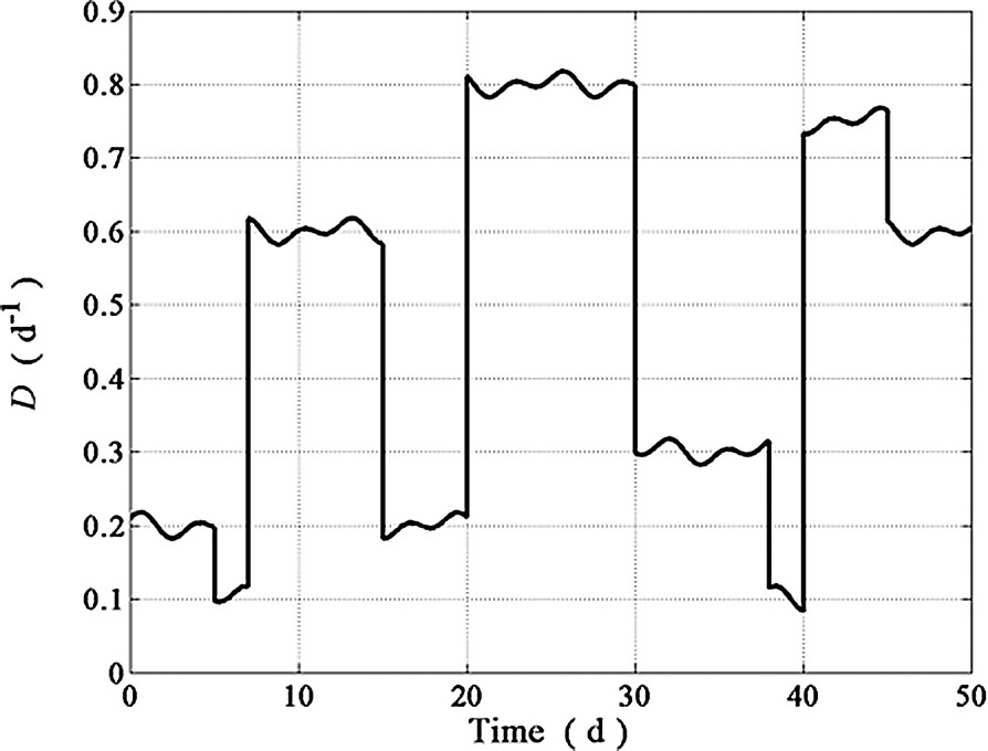
Dilution rate.
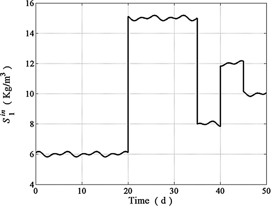
Influent COD concentration.
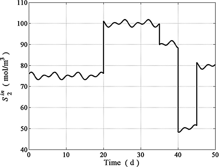
Influent VFA concentration.
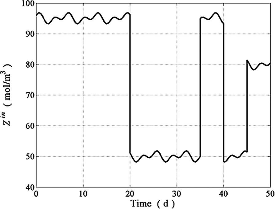
Influent strong ions concentration.
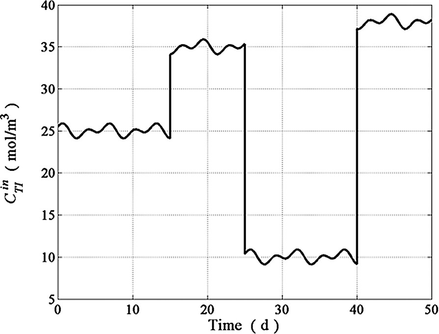
Influent total inorganic carbon concentration.

CO2 partial pressure profile.
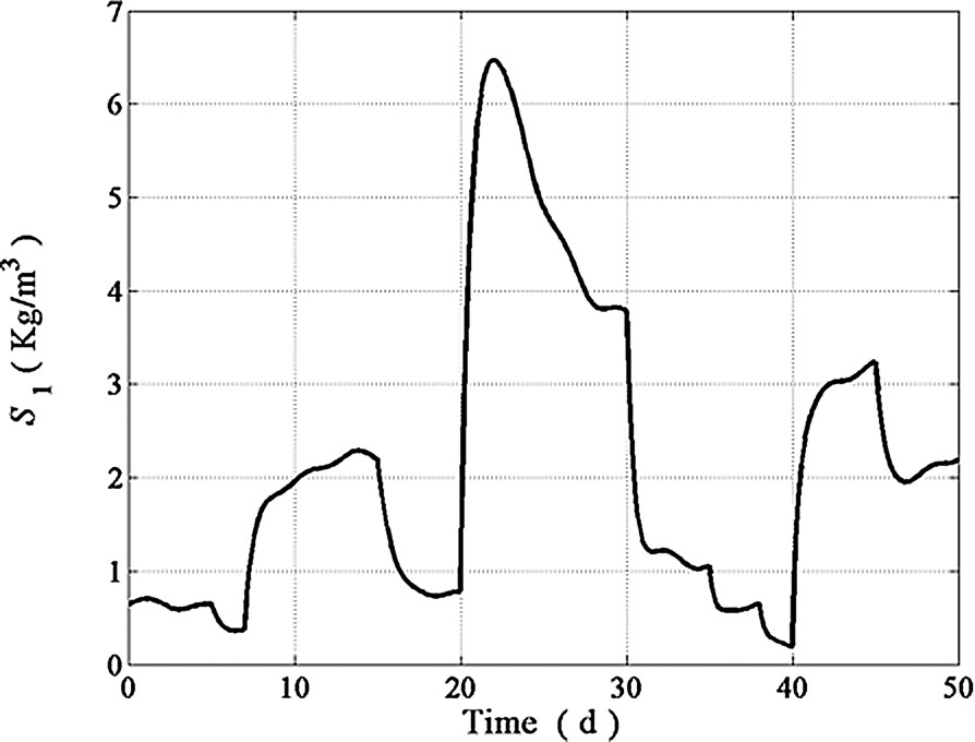
COD concentration.

VFA concentration.

Estimation of the acidogenic biomass concentration.
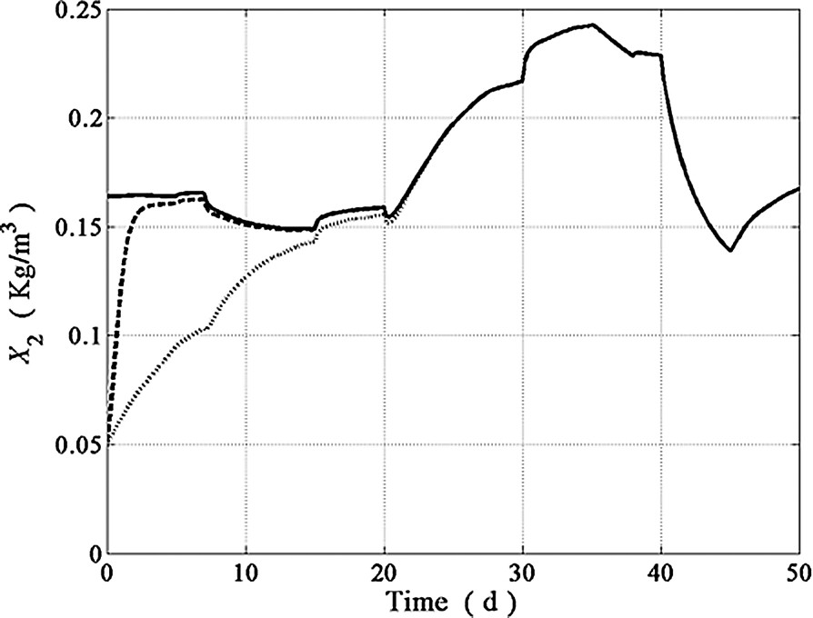
Estimation of the methanogenic biomass.

Estimation of the strong ions concentration.
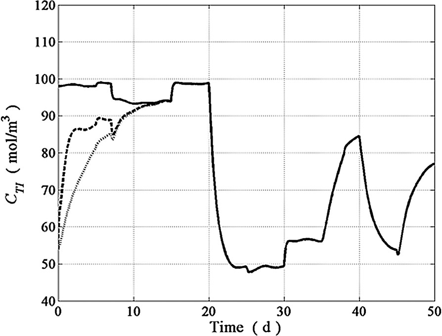
Estimation of the total inorganic carbon concentration.
6 Conclusions and perspectives
In this work, a robust asymptotic adjustable rate nonlinear observer for multidimensional biological systems has been proposed. It has been tested in numerical simulations on an anaerobic digestion process used in a wastewater treatment context. By using observer gains that were suitably chosen, this observer exhibited faster convergence rates than a classical asymptotic observer design. New studies are currently being conducted for optimizing the observer gains calculations. Because of the clear utility of this tuning observer in highly uncertain biological systems at the experimental scale, their use in robust nonlinear control schemes with application to continuous bioreactors is now under study.
Acknowledgments
The authors gratefully acknowledge to the ECOS-ANUIES Program (project: M97-B01), the CONACyT, the PROMEP Program and the European project TELEMAC (IST-2000-28156) for the support that made this study possible.


