

1 Introduction
Combining spectral and spatial information, Magnetic Resonance Spectroscopic Imaging (MRSI) provides distribution maps of metabolites. In standard experiments, the spatial information is obtained through phase encoding, requiring the acquisition of a number of scans at least equal to the number of voxels in the spectroscopic image. The spectral information is obtained through spin-echo or FID acquisition. In 1H MRS, due to the high number of metabolites that can be detected in the brain, the narrow spectral range (around 10 ppm) of their resonances, the multiplet structure of J-coupled resonances, and the line broadening caused by the inhomogeneities of the local B0 field, the peaks overlap, making quantification for mapping difficult.
Use of two-dimensional J-resolved spectroscopy is one way to avoid the peak overlap that 1D MRS suffers from. In 2D J-resolved spectra, the spectral information is spread onto a map: the chemical shift is encoded in the t2 direction and the J coupling in the t1 direction. It has been shown that 2D spectroscopic information can be combined with spatial encoding [1]. However, to obtain 2D spectroscopic images with high 2D spatial resolution, the acquisition time becomes excessive. For example, with a repetition time of 1 s, 32 encoding steps in both spatial directions, and 40 time increments, the minimum acquisition duration is longer than 11 h (without accumulation): this long duration strongly limits the biomedical use of such 4D techniques.
The minimum acquisition time of 4D SI can be reduced by using fast SI techniques based on various fast imaging solutions, including U-FLARE [2], echo-planar [3], multi-coil array [4] and spiral imaging [5]. Among these methods developed to reduce the minimum number of scans, the echo-planar SI based methods, for instance the Spiral Spectroscopic Imaging (SSI), use the delay between two successive time-domain points to sample spatial information. In SSI, the minimum acquisition time is reduced by applying a series of readout gradients during the acquisition window to collect simultaneously spatial and chemical shift information. Thanks to fast spiral encoding of the 2D spatial domain, the acquisition of t1 data can be achieved in a reasonable time. On the other hand, a good quality of the gradient hardware, a gridding algorithm and the measurement of the actual k-space trajectory become necessary to obtain a spectroscopic image.
We propose a k-space trajectory waveform based on continuous series of growing and shrinking (‘out-and-in’) spirals [6] instead of just growing spirals, as are usually used in SSI [7]. Adding to the advantages of spiral imaging, like symmetry of k-space apodization by transverse relaxation effects, symmetry of gradient hardware demands, etc., out-and-in spiral k-space trajectories increase the robustness of SSI against the artefacts of flow and motion thanks to its readout gradient moment nulling, and also avoid specific rewinding gradients to return to the centre of k-space.
We present a high-spatial-resolution 4D out-and-in SSI experiment performed on rat brain at 7 T, and the data processing necessary to reconstruct the spiral spectroscopic images. The quality of the image is evaluated by spatial-resolution estimation, and signal-to-noise measurement.
2 Method
2.1 Spiral spectroscopic imaging pulse sequence
During the rising (falling) part of each out-and-in spiral module, Nrot rotations are accomplished at constant angular velocity β = 4 π Nrot/T. The spiral radius increases or decreases linearly with time between 0 and kmax, at rate α = kmax/T [8]. A single rotation takes T/(2 Nrot) second, and the radius changes by kmax/Nrot at each turn. Using complex notation, the k-space trajectory curve (k(t) = kx(t) + i ky(t)) is described for a single out-and-in spiral module of duration T by:
| (1) |
A circular k-space region of diameter 2 kmax is covered (Fig. 1). Segmentation in k-space is achieved by the initial phase term 2 π s/Nk, where s = 0, ... Nk–1 is varied between acquisitions of the Nk k-space interleaves [9]. Ndat points were acquired during each spiral module.
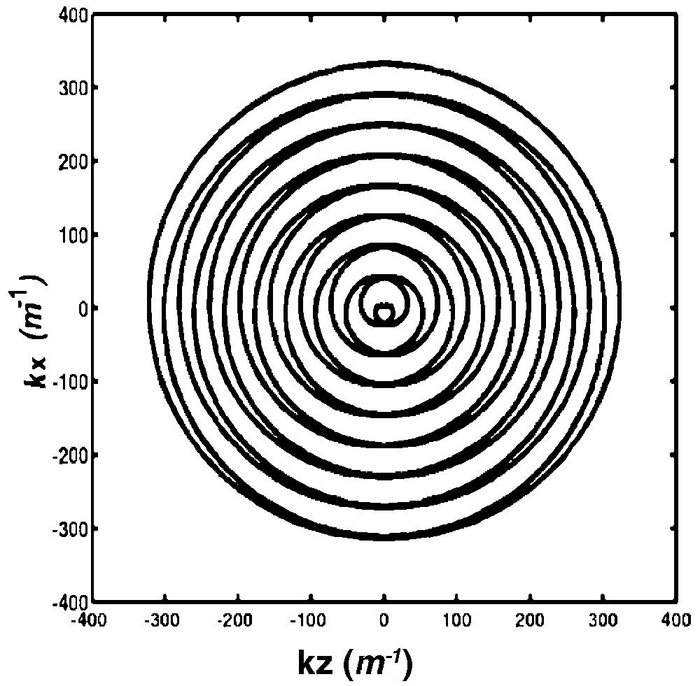
Description of k-space by one single out-and-in spiral module of Nrot = 8 turns. Each k-space interleaf starts at the centre, goes out to the boundaries, and then returns to the centre of the k-space.
In the t2 domain, to sample the information over a spectral bandwidth SW (inverse of the sampling time DW), a single spiral should start every DW. At high field, to cover the 10-ppm bandwidth (1H MRS spectral width), DW is shorter than at low field. Depending on the hardware limitations for gradient rise-time, it may be not possible to sample all the data associated with a particular k-space plane within such a short DW, so temporal interleaves may be required. Nspiral out-and-in spiral modules were applied after each excitation, and Nt2 temporal interleaves were acquired by delaying by DW the opening of the acquisition window and, therefore, the start of the spiral readout gradients (Fig. 2). A total of N = Nt2 Nk Nspiral Ndat points were thus sampled during Nt2 Nk excitations that encoded the kx, ky, and t2 domains. To describe the t1 domain, Nt1 increments were achieved by echo-time incrementation, leading to a total experiment time of Nt2 Nk Nt1 TR Na where TR is the repetition time and Na the number of averages. More details can be found in [6].

The complete echo signal was sampled during application of spiral readout gradients (= 1024 points acquired for each spiral). To ensure correct spectral sampling, temporal interleaves were used by shifting the beginning of the acquisition window by DW. For each temporal interleaf, Nspiral samples (red points) were acquired to describe the t2-dimension.
Before the out-and-in spiral readout gradients, the volume of interest (VOI) was selected with a PRESS (Point-Resolved Spectroscopy) sequence [10] (Fig. 3). The PRESS sequence was preceded by a CHESS (Chemical Shift Selective) module for water suppression [11] and an outer-volume-saturation (OVS) module to decrease spatial contaminations.
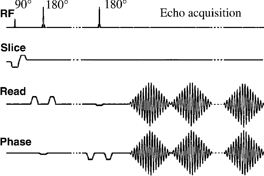
The spiral spectroscopic imaging sequence consists in a PRESS module followed by out-in spiral readout gradients (water suppression and outer-volume saturation modules not shown). The t1 domain was sampled by incrementing the echo time. The 180 slice-selective pulses were flanked by crusher gradients on read and phase channels.
2.2 Experiment and acquisition parameters
Experiments were performed on a SMIS console interfaced to a 7 T, 20-cm-diameter bore magnet (Magnex Scientific Ltd, Abingdon, UK), equipped with actively shielded Magnex gradients (MkSGRAD II, 200 mT m–1 max, 120 mm diameter) driven by gradient amplifiers Techron series 7700, with a maximum slew rate of 2 T m–1 ms–1. MR data were collected from rat brain using a homemade single-turn surface coil (diameter 25 mm) for RF pulse transmission and signal reception.
All procedures involving animals conformed to the guidelines of the French Government (decree No87-848 of 19 October 1987, licenses 006683 and A38071). Male Wistar rats (about 225 g) were used and anaesthesia was induced with 4% isoflurane in air (v/v) and then maintained with a mixture of 0.7–1.2% isoflurane in air enriched with oxygen to 30%. Rectal temperature was maintained at 36.5–37.5 °C by a regulated heating pad placed under the abdomen.
After obtaining scout-proton spin-echo images in transverse and coronal orientations, the PRESS VOI (15 × 18 × 3 mm3) was localized in a slice parallel to the coil (X, Z horizontal plane). The field of view was set to 30 × 30 mm2. After manual shimming in the VOI (about 25 Hz FWHM for the water signal), the OVS and CHESS parameters were adjusted. During an acquisition window of 81.92 ms, 8192 data points were collected applying Nspiral = 8 out-and-in spiral readout gradient modules after each excitation. k-space covering of 2 kmax = 666 m–1 in both kx and kz directions leads to a nominal spatial resolution of 1.5 mm. Using 2 k-space interleaves (Nk = 2) and Nrot = 8 rotations, the FOV was 48 mm, computed from the sampling interval on the k-space axes (32 points sampled on each axis). To achieve a f2 spectral bandwidth of 3125 Hz, Nt2 = 32 temporal interleaves were acquired by incrementing the duration between the last RF pulse of the PRESS sequence and the opening of the acquisition window by DW = 320 μs. Starting at an echo time of 100 ms, 16 increments of 30 ms were performed in the t1 domain resulting in a f1 bandwidth of 33.33 Hz. To encode the kx, kz, and t2 domains, an acquisition time of 2 min 40 s was required leading to a total acquisition time of 42 min 40 s (TR of 2500 ms).
2.3 SSI data processing
The k-space and the t2 domain were partially sampled after each excitation. Therefore, (kx, kz, t2) data of each t1 step were first re-ordered into {(Nspiral+1) Nt2 – 1} time intervals of DW. Within each interval, samples were thus acquired for times ti where:
| (2) |
For each (kx, kz) coordinate, a first-order phase correction was applied in the spectral domain to obtain the projection of the (kx, kz, ti) data onto (kx, kz, i DW) planes. This will result in {(Nspiral+1) Nt2 – 1} (kx, kz) planes regularly spaced in the time direction.
The Nt2 first and (Nt2 – 1) last temporal planes of each t1 step were rejected, resulting in a total of {(Nspiral – 1) Nt2} (kx, kz) planes in the t2 direction. This rejection was necessary because, in these first and last planes, the spiral had sampled only the centre of k-space, from one single point for the very first plane to an almost but not completely sampled k-space for the Nt2th one. Therefore, this insufficient sampling of k-space was likely to introduce some artefacts, and the corresponding planes were suppressed from the reconstruction.
In k-space, a gridding algorithm is needed for re-sampling the data of each temporal plane onto a Cartesian grid [12,13]. This was done as follows: (1) data were re-ordered according to spatial and spectral interleaving schemes; (2) FFT was done in the temporal domain followed by first-order phase correction in the spectral domain, and inverse FFT; (3) the temporal planes with insufficient sampling were rejected; (4) the spatial data were resampled onto a Cartesian grid with a Kaiser-Bessel interpolation kernel; (5) Hanning filtering and zero-filling points along both k-space axes, and 2D inverse FFT; the points outside the displayed FOV (30 mm) were discarded; (6) Hanning filtering, zero-filling and FFT in the t2 domain; (7) Hanning filtering, zero-filling and FFT in the t1 domain. All processing steps were performed with an in-house program in C. The metabolite images were computed by numerical integration of metabolite peaks all over the datasets.
The Kaiser–Bessel interpolation function used in the gridding step was computed with a window width L = 3 pixels of the Cartesian grid in both directions, and a half bandwidth product B = π L. The inverse of the sampling density compensation function necessary for the gridding algorithm [13] was calculated from the areas of the Voronoi diagram zones of the measured k-space trajectory.
3 Results
Digital resolutions of 6.1 Hz and 2.0 Hz per point were achieved in the f2 and f1 domains respectively. The resonances of N-acetylaspartate (NAA) at 2.0 ppm, glutamate/glutamine (Glu) at 2.4 ppm, creatine (Cre) at 3.0 ppm and choline (Cho) at 3.2 ppm were clearly observed on a 2D spectrum extracted from SSI datasets (Fig. 4). Fig. 5 shows the Cr (3.0 ppm) image computed from spiral spectroscopic datasets.
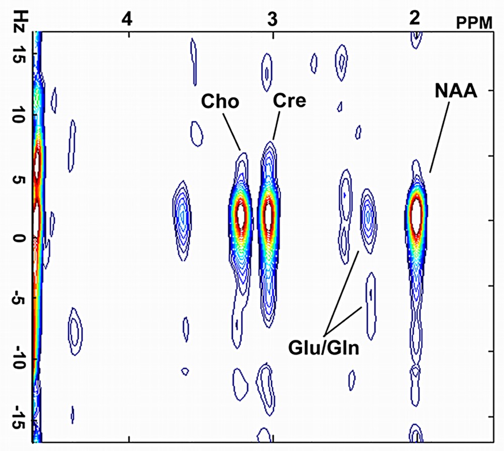
A 2D J-resolved spectrum extracted from a SSI dataset on rat brain.

(A) Proton spin-echo image corresponding to the slice in which the 4D dataset was acquired, with the contour (red box) of the volume-of-interest. (B) Metabolic image of Cr (3.0 ppm) from a rat brain in vivo from the 2D J-resolved 2D spatial dataset.
To evaluate the actual spatial resolution of the spectroscopic image, the theoretical point-spread function (PSF) was computed as a function of k-space sampling, gridding and spatial filtering (Fig. 6). The voxel size of the spectroscopic experiment was estimated to be 27.0 μl by numerical integration of the volume of the PSF function scaled to slice thickness.
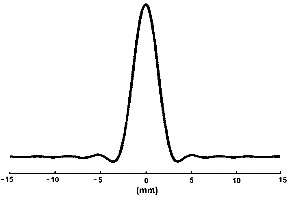
Theoretical point-spread function corresponding to the sampling and processing used for the out-and-in spiral spectroscopic image (one axis): the volume under the 2D PSF gives the volume of the voxel (27 μl).
The SNR was calculated from the intensity of the phased NAA peak divided by the noise r.m.s. measured between 6 and 8 ppm. For 10 pixels spaced by more than the PSF FWHM (3 mm) of the SSI dataset, the average SNR was 16.3 ± 4.6.
4 Discussion
An in-vivo 2D J-resolved spiral spectroscopic image with 16 steps in t1 and a 20 × 20 spatial matrix was achieved with a SNR higher than 16, in 42 min 40 s against 4 h 26 min for a standard phase encoding MRSI. The dependence of the PSF function on T2*, or on the chemical shift was not taken into account in the theoretical calculation, so the actual voxel size can be slightly larger than the 27 μl estimated from the SSI PSF.
The in-vivo high-resolution out-and-in SSI method combines high strength spiral readout gradients (up to 87.3 mT m–1) and rapid commutations (up to 0.83 T m–1 ms–1). This probably leads to a significant deviation between the theoretical and the actual k-space trajectories due to eddy currents, gradient system limits and pre-emphasis settings. To avoid all artefacts caused by this deviation, the actual k-space trajectory measured according to [14] was used to reconstruct the spectroscopic image.
Three-dimensional gridding was avoided by considering that the time-domain was regularly sampled throughout the data acquisition. First-order phase correction was used for data interpolation within a spectral dwell-time: gridding can be a time-consuming process, and our approach may be an advantageous alternative.
The k-space oversampling, resulting in a FOV of 48 mm, prevents the replica sidelobes produced by the gridding algorithm from being folded into the image of interest, and reduces the aliasing artefacts from the acquisition truncature. After the inverse FFT in the spatial domain, the data points outside of the FOV of interest were discarded, and only the data corresponding to a FOV of 30 mm containing the rat brain were kept and processed further.
Compared with standard spiral encoding, out-and-in spiral encoding somewhat increases the time efficiency of the sequence since all the data points collected in the acquisition window are used for image reconstruction. Moreover, thanks to the time symmetry of the gradient waveform, leading to periodically null gradient moments, the sensitivity to motion is further reduced, as recently demonstrated by Kim et al. [15].
5 Conclusion
We have demonstrated the feasibility of fast spiral 2D-spectral 2D-spatial spectroscopic imaging at high field in vivo. Mono-voxel clinical 2D spectroscopy has recently been proved useful for obtaining more information for spectral characterization and to better assign the resonances [16–18]. Robust rapid spectroscopic imaging techniques open the way to clinical applications of 2D spectroscopy.
Acknowledgements
The authors thanks R. Farion for the animal preparation, J.A. Coles and L. Lamalle for helpful discussions. B.H. received a grant from the ‘Association pour la recherche contre le cancer’. The NMR facilities were supported in part by the ‘Programme Interdisciplinaire Imagerie du petit animal’ (CNRS–INSERM, France)