

1 Introduction
Heteronuclear spin relaxation is being used increasingly to study the dynamics of proteins [1,2]. An incentive to these studies is the search for correlation between structure, dynamics and function [3,4]. A large number of such heteronuclear relaxation studies have focused on amide 15N–1H spin system in isotopically enriched protein samples [5,6], thereby allowing the local dynamics along the protein backbone to be explored residue by residue. Typically, dynamical information is derived from the longitudinal and transverse relaxation rates, R1 and R2, respectively, and also from the cross-relaxation (1H–15N) rate (denoted by σNH in the following).
The dynamic information content of the 15N heteronuclear relaxation rate constants consists of discrete evaluation of the spectral density functions J(ω) belonging to the various 15N–1H bonds. Peng and Wagner have proposed a strategy in which one measures a set of six relaxation parameters for the 15N–1H bonds at a given B0 field strength [7,8]. Nevertheless, random as well as systematic errors for some of the measured relaxation rates render accurate and precise determination of the values of J(ω) at high frequencies (J(ωH), J(ωH ± ωN)) difficult. By assuming a slow variation of J(ωH) around the proton frequency for low tumbling proteins, the “high-frequency approximation” allows a more accurate “reduced spectral density mapping” through the determination of J(0), J(ωN) and 〈J(ωH)〉 (the “average” value of J(ω) for ωH − ωN, ωH and ωH + ωN frequencies), with the measurement of only three heteronuclear relaxation rates, usually the longitudinal relaxation rate (R1), the transverse relaxation rate (R2) and the 1H–15N cross-relaxation rate σNH, usually obtained through the measurement of the heteronuclear [1H–15N] NOE [9–11]. Besides the gain of accuracy, this approach allows a considerable gain of experimental time, since only three relaxation rates instead of six need to be measured. The drawback of this method resides in a poor description of the spectral density function, which can be notably insufficient for the description of complex motions. A straightforward way to obtain a better description of the shape of density function is to measure 15N relaxation rates at multiple NMR fields: recording data at n field strengths will provide 2n + 1 discrete values of the spectral density, but at the expense of a very long measuring time, since 3n relaxation experiments must be recorded (n R1, n R2 and n [1H–15N] NOE experiments). We have recently proposed an alternative method based on an additional approximation that takes in account the very different relative contributions of the spectral densities at 0, ωN, and 〈ωH〉 frequencies to the longitudinal, the transversal, and the 1H–15N cross-relaxation rate in case of low tumbling proteins [12]. Within the validity interval of this approximation, n + 2 values of the spectral density function can be obtained by recording n + 2 relaxation experiments only, when using n different NMR field strengths: namely a single R2 relaxation rate and a single heteronuclear [1H–15N] NOE experiment at a given field strength, and a R1 relaxation rate for each NMR field strength. Owing to the considerable gain in experimental time, we have called this approach “fast spectral density mapping”. In the present manuscript, we demonstrate that this method is as robust as the conventional spectral density mapping methods to describe the complex internal motions experienced by the protein C12A-P8MTCP1.
P8MTCP1 is a disulfide-rich 68-residue (8 kDa) protein co-expressed with the oncogenic protein P13MTCP1. If its function remains still unknown, its robustness makes it a model of choice extensively used in our laboratory for methodological development purposes. As shown in Fig. 1, the solution structure of P8MTCP1 [13] reveals an original scaffold consisting of three α-helices, associated with a new cysteine motif. The core of the protein mainly consists of two helices (helix I: residues 7–20, and helix II: residues 29–40), which are covalently paired by two disulfide bridges (Cys38–Cys7 and Cys17–Cys28), forming a α-hairpin. A relatively well-defined loop (residues 41–47) connects helix II to helix III, which spans residues 50–65. The third disulfide bridge (Cys39–Cys50) links the top of helix III to the tip of helix II. Helix III is oriented roughly parallel to the plane defined by the α-antiparallel motif and appears less defined. Except for the first N-terminal turns, few NOE contacts were found between the third helix and the α-hairpin, suggesting that helix III is loosely bound to the core of the protein. In the recombinant C12A-p8MTCP1 mutant protein [14], an alanine residue has replaced the “free” cysteine residue at position 12 in the native sequence, to improve the expression yields in Escherichia coli.
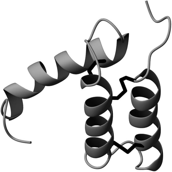
Ribbon diagram of the structure of C12A-P8MTCP1 showing the backbone and disulfide bonds.
2 Material and methods
2.1 Theory
When the relaxation of the 15N nucleus is predominantly caused by the dipolar interaction with its attached amide proton and by the anisotropy of its chemical shift, the relaxation data can be interpreted in terms of the motion of the 15N–1H vector. Given that the three experimentally determined parameters, RN(Nz), RN(Nxy) (denoted as R1 and R2, respectively, in the following) and NOE, depend on the spectral density function at five different frequencies [15], the calculation of the spectral density values can be approached by the application of the so-called reduced spectral density mapping, in which the relaxation rates are directly translated into spectral density at three different frequencies [7–11]:
| (1) |
| (2) |
| (3) |
If in the multi-field spectral density mapping approach, spectral densities are calculated from the relaxation rates R1, R2 and the NOE obtained for each given magnetic field induction value, a combination of relaxation rates obtained at different magnetic field inductions can be used for the fast spectral density mapping, as previously published [12]. Indeed, when using the spectral density approach to analyze relaxation data recorded at n NMR fields, the measurement of a complete set of relaxation parameters (R1, R2 and NOE) for each magnetic induction value is requested, yielding n values of J(ωN), n values 〈J(ωH)〉, and only one value of J(0). If one discards the possible contribution of exchange contributions that will be discussed later, it appears that the information on J(0) is highly redundant, since this spectral density value is independent of the magnetic field induction value. Hence, the information on this particular point on the spectral density function can be readily obtained through the measurement of the 15N heteronuclear relaxation parameters at a single NMR field value. Moreover, if we limits ourselves to the case of low tumbling proteins, where R1, R2 and σNH currently differ from each other by about an order of magnitude, Eq. (1) shows that the J(0) values are largely dominated by the R2 values, with a non-negligible contribution of R1 values when ωτc decreases, and a merely negligible contribution of σNH. As a result – and as it has been previously checked by simulations [12], if the measurement of R2 and R1 needs to be done at the same NMR field, the NOE value used in Eq. (1) can be obtained at a different frequency without altering significantly the resulting value of J(0).
Furthermore, we have previously demonstrated [12] that a good description of the Lorentzian function around J(ωN) can suffice to discriminate between the different kinds of motions: it is thus possible to restrict the information on the spectral density at high frequency to one point. As a result, a single set of NOE and R1 measurements can suffice to obtain the value of 〈J(ωH)〉. Contrary to J(0), and because the value of 〈J(ωH)〉 depends (and depends only) on the product NOE × R1, these two relaxation rates must be recorded at the same NMR field: thus, the value obtained for 〈J(ωH)〉 corresponds to its exact value, within the high frequency approximation limits. Then, an extensive sampling of the spectral density around J(ωN) can be obtained through the measurement of R1 rates only, at each NMR magnetic field. Indeed, Eq. (2) shows that the J(ωN) value is essentially dominated by R1, with – in case of low tumbling molecules – only a weak contribution of σNH. Thus, the n J(ωN) values – corresponding to the n different magnetic field strengths – can be obtained through the measurement of the corresponding R1 rates only: the NOE value used in Eq. (2) will be the same for all NMR magnetic fields, the one already used for the calculation of 〈J(ωH)〉. As a result, the exact value of J(ωN) is obtained only for the magnetic field strength where both R1 and NOE are measured. Previous simulations have shown only a weak deviation from the exact value for the other magnetic induction values [12].
Then, assuming that 1H–15N vectors are animated by a more or less complex combination of diffusive motions, and that C12A-P8MTCP1 tumbles isotropically, we used the following models to analyze the spectral density functions:
| (4) |
| (5) |
| (6) |
| (7) |
| (8) |
| (9) |
2.2 Experimental
Heteronuclear relaxation parameters have been previously obtained at five magnetic field strengths ranging from 9.4 T to 18.8 T (corresponding to proton frequencies of 400, 500, 600, 700 and 800 MHz), on an 15N-uniformly enriched 400 μM sample of C12A-p8MTCP1 dissolved in 25 mM phosphate buffer, 50 mM NaCl, at pH 6.5. The temperature was carefully adjusted using a calibration sample (80% glycol in d6-DMSO) and set to 20 °C. Details on the protein expression and purification, as well as on the parameters used for the relaxation experiments, can be obtained from previously published papers [14,16].
Each individual set of J(ω) values was then fitted with either the Lipari–Szabo or the extended Lipari–Szabo models with our in-house written program DYNAMOF (www.cbs.cnrs.fr) [22]. In the SIMPLEX optimization process, only the τc value was fixed, and the S2, Ss2, Sf2, τs and τf values were tentatively optimized starting from identical guess values whatever the model used.
3 Results and discussion
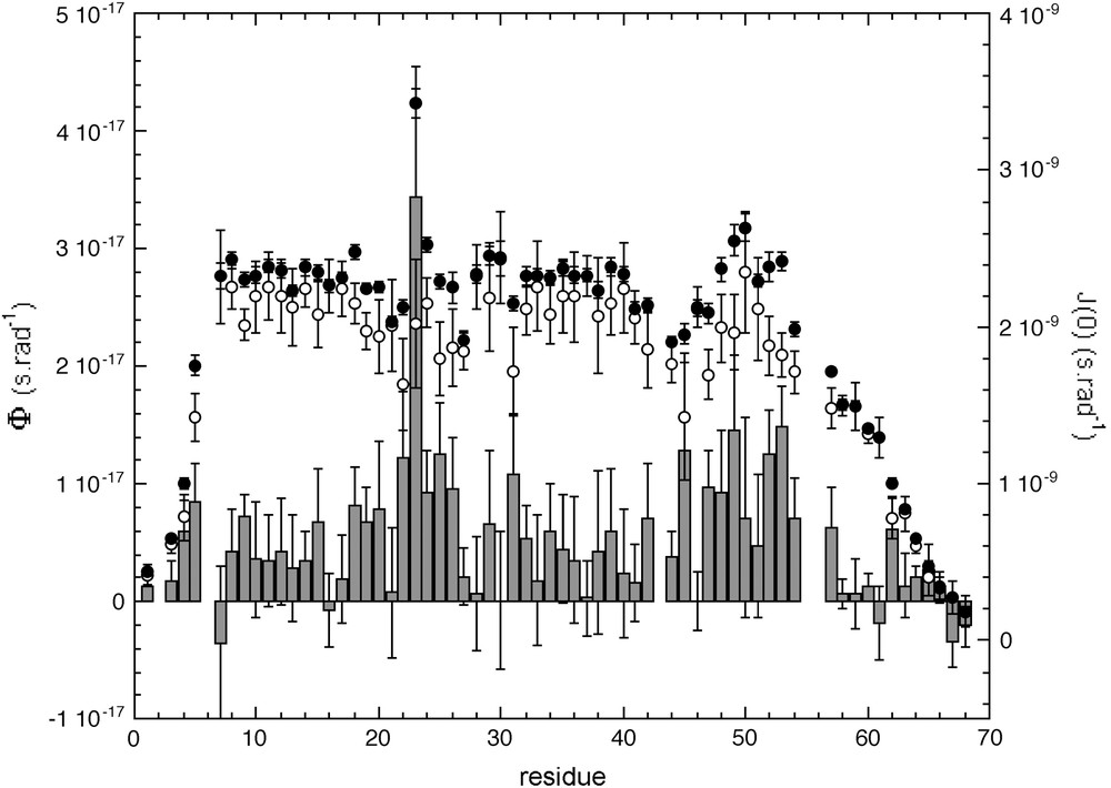
Fig. 2 shows the R2, R1 relaxation rate constants and the heteronuclear NOEs at stationary state that were measured for most of the non-proline residues of C12A-p8MTCP1 at five different magnetic field induction values, as well as the corresponding reduced spectral densities J(0), J(ωN) and 〈J(ωH)〉 obtained from the reduced relaxation matrix (Eqs. (1–3)). The spectral densities for the NH vectors clearly show a different behavior in the α-hairpin than in helix III: whereas the spectral density values remain on a plateau for helices I and II, they display a monotonic decrease from the N- to the C-terminal end of the helix. This indicates an increasing contribution of high-frequency motions. As suggested by lower values for J(0), the loop connecting the α-hairpin to helix III is expected to be more flexible than helices I and II, but appears more rigid than the C-terminal turns of helix III. Finally, most of the residues in the two interlocking turns (residues 21–28) connecting helix I to helix II show lower J(0) values than in the rest of the α-hairpin, with a concomitant increase of the J(ωN) and 〈J(ωH)〉 values. This reflects the higher flexibility of these turns as compared to the helices in the α-hairpin. In this area, Tyr23 shows significantly higher values of J(0), especially when calculated with relaxation parameters measured at high field, while J(ωN) and 〈J(ωH)〉 for these residues are not smaller than the mean values. This strongly supports the hypothesis that slow movements in the micro- to millisecond range exist in this loop.

(Left) Relaxation rate constants and 15N{1H}NOEs, as a function of the protein sequence, measured at 9.4 T (filled circles), 11.75 T (open circles), 14.1 T (filled triangles), 16.45 T (open triangles) and 18.8 T (filled diamonds). The relaxation rate constants R1 and R2 were obtained from non-linear fits of peak heights to monoexponential functions. The uncertainties were determined from 500 data sets generated according to the Monte Carlo procedure. The 15N{1H}NOE is deduced from the ratio of peak heights obtained with and without proton saturation. (Right) Spectral density functions, as a function of the protein sequence, obtained from relaxation rates measured at 9.4 T (filled circles), 11.75 T (open circles), 14.1 T (filled triangles), 16.45 T (open triangles) and 18.8 T (filled diamonds). The “conventional” spectral density mapping (SDM) has been used for calculation.
The mapping of spectral densities J(ω) for each backbone NH bond provides the intrinsic dynamic information from the relaxation data – without any assumption for the motional model – upon which a variety of motional models may be evaluated. Since both values of J(ωN) and J(ωH) decrease for almost all NH vectors with increasing frequencies ωN and ωH, respectively, the description of the spectral densities as sums of Lorentzians' appears qualitatively reasonable for C12A-p8MTCP1. Adequate fits of J(ω) are therefore expected using the model-free formalism proposed by Lipari and Szabo [17]. The combination of relaxation data sets from five different magnetic fields resulted in seven or eleven independent values of the spectral density function per NH bond when using fast or “conventional” spectral density mapping, while a maximum of only four parameters using Eq. (5) (non-simplified “extended” Lipari–Szabo model) is required to model J(ω), giving a substantially high number of degrees of freedom. On the other hand, the ratio of the principal components of the average inertia tensor for the backbone atom on the average structure of C12A-p8MTCP1 was determined to be 1.24 [23,24]. This number suggest that the overall rotation of the protein is expected to have only a small degree of anisotropy that may not have a strong influence at least on the order parameters' values [25]. Thus, we do not make any attempt to introduce this contribution in the motional model.
Spectral densities were calculated and fitted with the Lipari–Szabo model using DYNAMOF. To assess the validity of our strategy, three different protocols were considered.
- 1. After calculation of J(0), J(ωN) and 〈J(ωH)〉 using the conventional spectral density mapping approach, the J(0) values were tentatively corrected from exchange contribution using Eqs. (7 and 8). J(0)cor, J(ωN) and 〈J(ωH)〉 values were then fitted using Eqs. (4–6).
- 2. In the second protocol, J(0) values were not corrected: exchange contributions were obtained by an additional fit of the raw spectral densities with Eq. (9).
- 3. In the third protocol, the fast spectral density mapping approach was used to calculate J(0), J(ωN) and 〈J(ωH)〉. We chose to use the same field for measuring R2 and NOE (14.4 T), contrary to what we did in a previous report (and on a different protein) where R2 and NOE were measured at the lowest field and at the highest field, respectively. This yields two “exact” values for both J(0) and 〈J(ωH)〉, instead of only one (〈J(ωH)〉) with the previous combination. Of course, R1 values measured at each individual field were used for the calculation. The spectral densities were then fitted with Eqs. (4–6) and (9).
A common first step for the three protocols was the calculation of the “global” tumbling time value τc, common to all residues in the protein. This was achieved by fitting the spectral densities with Eq. (4) (“simple” Lipari–Szabo model), where τc, S2 and τ were used as adjustable parameters. A mean value as well as a standard deviation was then calculated for τc over all the residues in the sequence: residues for which were excluded and the remaining residues were used for a second fit. This procedure was iterated until 67.5% of the residues fell into a ± 2σ interval value. Thus, τc values of 5.94 ± 0.20 ns, 6.29 ± 0.28 ns and 6.51 ± 0.14 ns were obtained when using protocols 1 (correction of J(0) values), 2 (“conventional” spectral density mapping (SDM)) and 3 (fast spectral density mapping (FSDM)), respectively. Whereas the τc values obtained with both SDM and FSDM are virtually identical, the first protocol gives a significantly lower value. This is due to the correction of the J(0) from the exchange contribution using the Φ value calculated with Eq. (7): as usually observed with this method, significant exchange contributions are observed for almost all backbone NH bonds (Fig. 3), yielding significantly lower values of J(0) after correction.
J(0)cor (open circles) and ϕ values obtained with protocol 1: J(0)cor values are obtained from the observed J(0) value corrected from exchange contributions using Eqs. (7) and (8). The average value of J(0) obtained for the five different magnetic fields are plotted as bold circles, ϕ values are plotted as bars.
Once the overall tumbling time τc has been determined, model-free parameters were obtained by using either the “simple” (Eq. (4) or the “extended” (Eq. (6)) Lipari–Szabo formalisms. We tentatively use the “non-simplified extended” Lipari–Szabo model (Eq. (5)), introducing τf as fourth additional parameter for the fit, but this procedure did not give significant improvements. On the other hand, an additional fit was performed in protocols 2 (SDM) and 3 (FSDM) with Eq. (9) in order to take into account possible exchange contributions to J(0). The physical relevancy of the microdynamic parameters (essentially S2 and τf) obtained from the different fits was used first to choose the “right” model, rather than the classical χ2 analysis. Indeed, since no “physical” limit value is imposed by DYNAMOF to the parameters in the fit, extremely good χ2 values can be obtained with irrelevant parameter values (for instance S2 > 1). As demonstrated in Fig. 4, this appears to be an easy and robust procedure for the selection of the “best” fit. Interestingly, for a given residue in the protein sequence, the best fit was obtained with the same equation whatever the protocol used, with some exceptions only in “boarder” regions of the molecule. These exceptions stem from the fact that it is difficult to discriminate between a combination of a slow and a single highly restrained (S2 ≈ 0.9) motion in the picosecond time scale, and a combination of a slow and two highly restrained (Sf2 × Ss2 ≈ 0.9) motions, even if the latter ones are on different time scales (pico- and sub-nanosecond). Interestingly, relevant S2 values (<1) was obtained for residue Tyr23 only when using Eq. (9) in the SDM and FSDM protocols: virtually identical ϕ values of 28.8 ± 2.87 × 10⁻¹⁸ s rad−1 and 26.9 ± 2.89 × 10⁻¹⁸ s rad−1, respectively, were obtained. When using Eq. (7), a comparable value of 34.37 ± 1.11 × 10⁻¹⁸ s rad−1 was obtained. When using this last approach, Tyr23 is the only residue that exhibits a significant value for ϕ (>mean value + 2σ), suggesting that exchange contributions should be considered only for this residue.
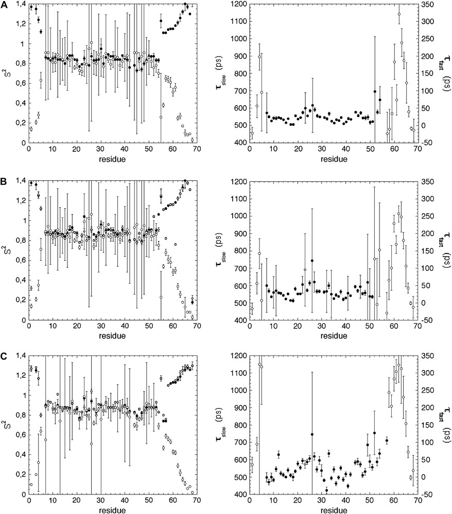
Generalized order parameters (S2) (left) and correlation times (τf and τs) (right) obtained when using the different Lipari–Szabo models (Eq. (4): filled circles; Eq. (6): open circles; Eq. (9): open diamonds) for the adjustment of spectral densities calculated with (A) protocol 1 (use of J(0)cor); (B) protocol 2 (“conventional” spectral density mapping approach (SDM)); (C) protocol 3 (fast density mapping approach (FSDM)). For the seek of clarity, only correlation times obtained from models giving relevant S2 values (<1) are reported.
The generalized and partial parameters S2, Sf2, Ss2 calculated with the three protocols (preliminary correction of J(0), SDM and FSDM) are reported in Fig. 5. Virtually identical values of generalized (S2) or partial (Sf2, Ss2) order parameters are obtained with SDM and FSM, whereas the corresponding values are slightly weaker when using the first protocol again, this can be attributed to the weaker J(0)cor values used for the fit in this protocol. Similarly, τf and τs values are on the same rank order for whatever the protocol used (see Fig. 4).
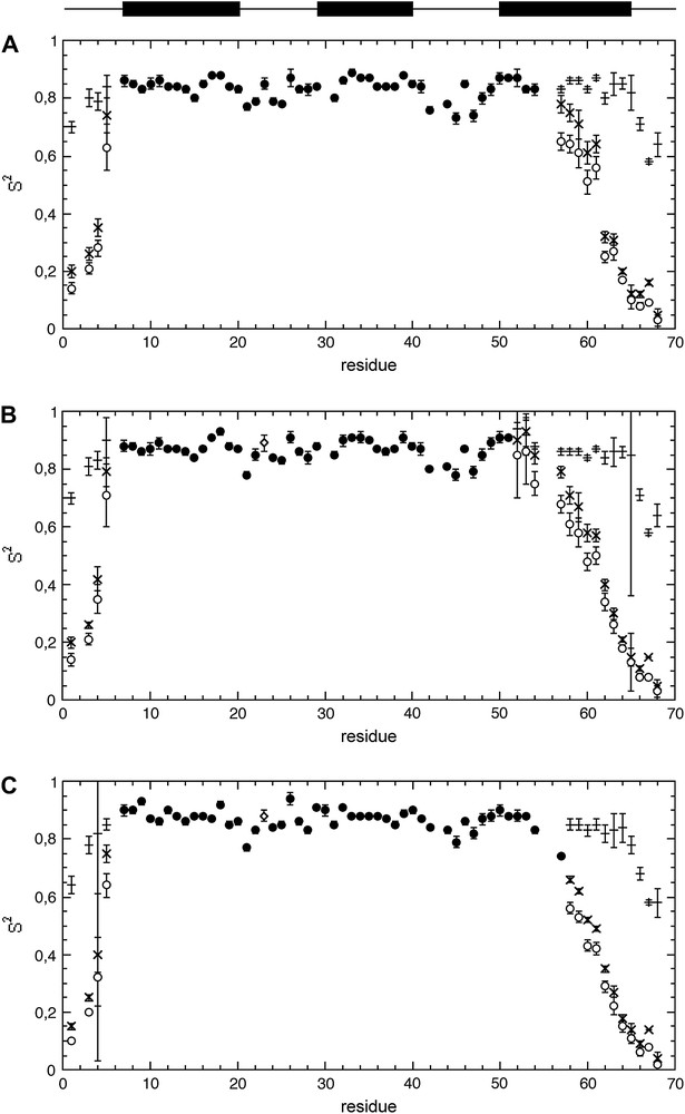
Results of the Lipari–Szabo analysis of spectral densities obtained with (A) protocol 1 (use of J(0)cor); (B) protocol 2 (“conventional” spectral density mapping approach (SDM)); (C) protocol 3 (fast density mapping approach (FSDM)). Generalized order parameter S2 are reported as filled circles, open circles, or open diamonds when obtained with the “simple” Lipari–Szabo model (Eq. (4)), the extended Lipari–Szabo model (Eq. (6)), or with the simple Lipari–Szabo model with correction of the exchange contribution (Eq. (9)), respectively. The symbols (+) and (x) stands for the partial order parameters Sf2 and Ss2, respectively. The secondary structure elements are schematized above the data.
Analysis of the microdynamic parameters – whatever the protocol used – shows the contribution of highly restrained (S2 ≈ 0.85) fast motions to the intrinsic dynamics of the α-hairpin (helices I and II) (Fig. 5). But an additional sub-nanosecond motion is necessary to fully describe the dynamics of helix III. The monotonic decrease of S2 values observed for this helix from the N- to the C-terminal is essentially due to a decrease of Ss2, the amplitude of the fast internal motion remaining highly restrained, as indicated by the high (≈0.85) and constant value of Sf2. This strongly suggests a sub-nanosecond hinge motion for helix III, with increasing effects on the generalized order parameter S2 when going from the anchoring point of the helix (the α-hairpin) to the “free” C-terminal end. This hinge motion can be easily differentiated from totally disordered motions as those present in the N- and C-terminal end of the protein: in this case, the decrease observed for S2 is due to the concomitant decrease of both Sf2 and Ss2, suggesting a concomitant increase of the amplitude of both the fast and the sub-nanosecond motions.
4 Conclusion
We have demonstrated that the association of the “model-free” analysis with our recently published fast spectral density mapping strategy gives virtually identical results as when model-free is associated with the regular spectral mapping density, as previously proposed by Wagner and Peng [26]. This remains true even in the case of the use of a very complete set of relaxation data, as the one obtained for C12A-P8MTCP1 where relaxation parameters were recorded at five B0 magnetic field inductions. Nevertheless, whereas the regular spectral mapping density needed approximately 10 days (≈12 h by R2 and R1 experiments, ≈24 h by NOE experiments) for measuring the complete relaxation data set at each B0 field (5 R2, 5 R1 and 5 NOE), the measurement time can be reduced to about 4 days with our new strategy (1 R2, 5 R1 and 1 NOE). By the way, we hope that this method will help to “democratize” the use of multiple-field relaxation approaches for the fine analysis of protein dynamics.
It should be noticed that since the model-free approach uses analytical expressions of spectral densities, their initial extraction is not a necessary step, and fits could be directly performed on the measured relaxation rates at different magnetic fields. Nevertheless, we have shown in a previous paper [12], that the initial calculation of spectral densities from relaxation rates relies on very reasonable assumptions, and gives in turn a very useful pictorial description of the intrinsic dynamics of the protein. Moreover, although qualitative, this description is completely “model-free”, contrary to the more quantitative one given by the improperly called “model-free” approach of Lipari–Szabo that needs some prerequisites on the nature of the motions (uncorrelated global and internal motions, isotropic tumbling).
Acknowledgements
Virginie Ropars is granted by the “Ligue contre le cancer”. The study of the oncogenic proteins from the TCL1 family is supported by the “Association pour la recherche contre le cancer” (France).