

1 Introduction
Ligand cone angles were introduced by Tolman to measure the size of phosphine derivatives and other phosphorus ligands [1]. This size is the solid angle defined by the smallest angle cone having its apex lying at 2.28 Å from the phosphorus atom and circumscribing the ligand atoms, usually modelled by spheres. The solid angle, expressed in steradians, is , where α is the angle between the generatrix of the cone and its axis (see general definitions in Section 3.1). In the case of symmetric ligands PR3, the Tolman cone angle is easy to compute because its axis is in the direction of the mean of the three vectors defined by the PR bonds. Then, given the radius of the spherical ligands, α is retrieved by elementary geometry calculus. This approach has to be refined for unsymmetrical ligands such as MPR1R2R3 and more generally for MXR1R2R3, where M = H or is a metal atom, and X = P, N, CH, or is any atom having a tetrahedral hybridisation such as sp3 or sd3. It was pointed out that even symmetrically substituted bulky phosphines may offer unsymmetrical conformations [2]. The difficulty of the calculation arises (i) when the spheres radii are unequal, and (ii) when the XRi bonds are not symmetrically arranged around the MX axis. Tolman approximated θ as , where is the acute angle between the directions of the XRi bond and of the MX bond [3,4]. This method was criticized because the obtained values may not reflect the properties of the ligand, particularly when the substituent groups differ greatly [5]. It seems that few geometric tools are available to measure steric effects in organometallic chemistry, and that could explain why ligand cone angles were much used in this field [6–9], Recently, Bilbrey et al. [10–12] proposed an analytic solution to the ligand cone angle calculation.
It was also proposed to measure the steric size of ligands and substituents by the solid angle generated by the union of the atomic spheres [13], rather than the one generated by their enclosing cone. This approach gives rise to an analytical calculation of the solid angle, provided that the intersections of more than two spheres could be neglected [13]. There is a non-linear relationship between the cone angle and the solid angle, which was measured quantitavely [14]. To evaluate the importance of sphere overlaps, an exact analytical calculation of sphere intersections was done with the ASV freeware [15] using the atomic radii recommended by Gavezzotti [16], and showed that intersections between 6 or 7 atoms are commonly observed in organic molecules [15,18]. These atomic radii are sometimes slightly larger than those given by Bondi [17], but it is recalled that an increase in the sphere radii does not guarantee an increase of the van der Waals surfaces. Running ASV on a database of 70 diverse ligands showed that neglecting the intersections of more than two atoms induced a mean error on van der Waals surface calculations of 249%, and that neglecting the intersections of more than three atoms led to a mean error of 87%, and neglecting the ones of more than four atoms led to a mean error to 16%, the maximal observed error in this case being 37% [18]. Despite that van der Waals surfaces are not used in ligand solid angles calculations, these numbers show the importance of atomic spheres overlaps.
An improved ligand solid angle algorithm was proposed, which takes into account spheres intersections of orders 3 and 4 [19], but it needs a complex numerical integration. Recently, Bilbrey et al. [12,20] proposed an analytic solution to the solid angle calculation, based on the decomposition of the solid angle contributions between those due to spherical polygon parts and those due to the resulting truncated spherical sectors parts. This algorithm, implemented by the authors in their Mathematica FindSolidAngle package, is effective for the simple geometrical arrangements expected to be encountered in chemistry. However, it is not specified how it works in general. E.g., the detection of potential multiple connected components got by projection at the surface of the unit sphere is not evoked, the solid angle subtended by an internal spherical polygon may be not void and may even be not unique, etc. The detection and the management of such situations let the algorithm rather difficult to implement.
The impact of conformational variations was evoked early [21], leading to use weighted average cone angles [22], while it was considered that this problem was overcome by the use of the solid angle methodology [23]. At the same time, Müller and Mingos noticed also that the Tolman cone angle definition does not take into account the variations due to conformational changes [24,25], and they used the atomic centers of the ligand atoms rather than their van der Waals spheres. Then they applied their algorithm to perform statistics on thousands of phosphine structures found in the Cambridge Crystallographic Data Base [26], and observed a variation in cone angles for specific ligands, which is much larger than had previously been suspected.
This slight change in the ligand cone angle calculation, that we retain here (see Fig. 1) offers two other major advantages: (i) the cone angle can be generalized to complex polyatomic ligands Ri via the calculation of the fixed apex minimal cone enclosing any desired number of atoms, and (ii) this calculation can be done analytically, as shown in Section 3 of the present paper. We emphasize that this generalization allows us to model molecular shapes and structural fragments with cones although it is usual to work with spherical models. Despite that is easy to compute spherical shapes, the spherical model was shown to be unrealistic and a cylindrical model was preferred for drug design applications [27]. Fortunately, minimal height enclosing cylinders and minimal radius enclosing cylinders are computable analytically [28]. However, it seems that apart cylinders and cones, it is hard to find the use of non-spherical molecular shapes in the literature: it may be due to the lack of simple analytical calculation algorithms.
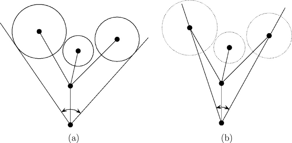
(a) Ligand cone, defined by Tolman [1]. (b) Smallest enclosing cone, defined here.
There are several ways to take into account the conformational changes of the ligands. We propose the following one. For each conformer, we know from the present analytical minimal enclosing cone algorithm which ligand atom centers are on the surface of the cone (see Section 3.5). We mark the atomic centers of these ligand atoms. These marked ligand atoms can differ from one conformer to another conformer, even for simple ligands such as Me or Et. Then, assuming a common origin in M, we are left with the problem of finding the best cone of fixed apex fitting all the marked atomic centers. We give in Section 3.3 an analytical solution to this problem, formulated as a least squares one. Then we define in Section 3.4 the conicity index κ, which takes values in the interval [0,1], the value κ=0 meaning that all marked atomic centers lies on the surface of the cone, and the value κ=1 being reached in the worst cases, characterized in Section 3.4. It is emphasized that, compared to our best fitting cone algorithm, computing some mean cone angle such as the arithmetic mean of individual cone angles, has drawbacks: such mean cone angle does not produce a mean axis, and computing some mean axis would not be coherent with the arithmetic mean of the cone angles. Furthermore, such a method would not permit to define a conicity index, although this latter provides quantitative information about the impact of conformational changes on steric effects. The axis of the best fitting cone is of interest because it gives rise to a second quantitative parameter: the acute planar angle between the axis of the smallest enclosing cone and the axis of the best fitting cone. This parameter indicates how the ligand size of MXR1R2R3 deviates from the mean ligand size of the family. At the opposite of the well-known RMS (Root Mean Square) deviation, it does not need the knowledge of a mean conformer.
A minor problem is to suppress the impact on a best fit cone calculation of free rotations around the MX axis before aligning the conformers in a common Cartesian coordinate system. When R1, R2 and R3 are different, a 3D rotation performed to optimally superpose each conformer on a common reference conformer solves the problem. It is proposed to set the pivot at M and to restrict this optimal rotation to X and to the respective three atoms of R1, R2 and R3 that are bonded to X, rather to involve more atoms when the Ri are polyatomic. The reason is that extending the optimal superposition to more atoms may give poor alignments in the neighborhood of X in the case of bulky ligands, while for usual applications of cone angles the neighborhood of X is assumed to be more important than the rest of the ligands. Furthermore, the restriction to X and to its neighbours permits potential extensions to superpositions of different molecules MXR1R2R3 rather than to different conformers of a common molecule MXR1R2R3, thus generalizing the definition of the best fitting cone. After translating the M atom of each conformer at the origin, each desired optimal 3D rotation can be found by minimizing the RMS deviation by the least squares method implemented in the ARMS freeware, which is based on quaternions (see appendix in [29], or appendix A.5 in [30] for more general results about optimal rotations). When two or three ligands are identical, there are respectively two or six pairwise correspondences between the ligands atoms bonded to X. In this situation, the one with the smallest minimized RMS is retained.
2 Results and discussion
We exemplify our minimal enclosing cone algorithm using a family of palladium triphenylphosphines complexes (Table 1). The resulting cone is equivalent to the Tolman cone for null atomic radii. The angle values we got are in the range 57.7–64.6°, and should be compared with the half of the Tolman cone angle values, which ranged in the interval 150.3–173.6°. This difference of a factor 2 is due to our mathematical definition of the cone angle, which stands in Ed (see Section 3.1).
Minimal enclosing cone angles for a family of palladium triphenylphosphines complexes. α: angle between the axis and the generatrix. θ: solid angle of the cone.
| Palladium complex (data from ref. [10]) | cos α | α (degrees) | θ (steradians) | Cone angle from ref. [10] | |
| 1 | Pd(PPh3) | 0.441571 | 63.796 | 3.509 | 170.0 |
| 2 | Pd(PPh3)2(SN2C3)2Cl | 0.532900 | 57.798 | 2.935 | 150.3 |
| 3 | Pd(PPh3)2(SN2C3)2Cl | 0.521229 | 58.585 | 3.008 | 155.4 |
| 4 | Pd(PPh3)(P2OC14H9)Cl | 0.534833 | 57.667 | 2.923 | 151.4 |
| 5 | Pd(PPh3)(SN4O2C8H7)Cl | 0.514252 | 59.053 | 3.052 | 155.2 |
| 6 | Pd(PPh3)(SN3C9H10)Cl | 0.501834 | 59.879 | 3.130 | 156.9 |
| 7 | Pd(PPh3)(SH) | 0.483577 | 61.081 | 3.245 | 160.8 |
| 8 | Pd(PPh3)2(S3NO2C7H5) | 0.489504 | 60.692 | 3.208 | 160.9 |
| 9 | Pd(PPh3)2(S3NO2C7H5) | 0.434539 | 64.244 | 3.553 | 173.6 |
| 10 | Pd(PPh3)(SNC5H4) | 0.474321 | 61.685 | 3.303 | 163.1 |
| 11 | Pd(PPh3)(NFC15H15)Cl | 0.485598 | 60.948 | 3.232 | 165.9 |
| 12 | Pd(PPh3)(SN3C10H11) | 0.458999 | 62.677 | 3.399 | 167.4 |
| 13 | Pd(PPh3)(S2N3C8H9) | 0.458199 | 62.729 | 3.404 | 167.7 |
| 14 | Pd(PPh3)(SN4C8H10) | 0.451533 | 63.158 | 3.446 | 170.6 |
| 15 | Pd(PPh3)(NFC11H15)Cl | 0.429580 | 64.559 | 3.584 | 172.2 |
The observed correlation coefficient between the ligand cone angle in [10] and our minimum enclosing cone angle α is rα = 0.9800, and with our solid angle θ is rθ = 0.9796, while α and θ are highly correlated (0.99995). Since the ligand cone angles encountered in the literature are almost all times used for empirical correlations with physical data, it is simpler to calculate α rather than the usual ligand cone angles because there is no need for atomic radii. The correlation between α and θ is not surprising because θ is a function of α. Then, the high value of the correlation coefficient indicates that the relationship can be estimated as linear for the considered ligands.
Published values of ligand cone angles are close to 180° (see Table 1) and can be greater than 180° for some nickel or platinium complexes [10], while 2α is around 120°. This difference is due to the exclusion of the ligand atomic spheres in the calculation of α. On the other hand, modeling the molecular shape by a cone should either take in account all atomic spheres, including the one of the metal (estimated to 1.63 Å for Pd [17]), or ignore all atomic spheres. Locating the apex of the cone enclosing all atomic spheres (including the metal one) would lead to a complex algorithm, and worse, would need the knowledge of adequate atomic radii. Ignoring only the atomic sphere of the metal gives large angle cones, close to a half plane, which are not realistic from the molecular shape point of view. Ignoring all atomic spheres leads to a very simple analytical algorithm (Section 3.5), it does not require atomic radii, the angle values are still pertinent for establishing empirical calculations, and the conical molecular shape is physically more realistic than a half plane. E.g., for the tetrakis Pd(PPh3)4 a solid angle close to 0.5 half space per Pd(PPh3) part is more realistic than a solid angle around one half space because for this latter the sum of the four contributions of the Pd(PPh3) parts is around two full spaces, thus indicating excessive cone intersections.
In order to define a mean cone for the 15 complexes of Table 1 and to evaluate quantitatively the dispersion around this mean cone, we operated as follows. The mean cone has sense only in a common Cartesian coordinate system: we selected Pd(PPh3) (see Table 1) as the reference complex to perform a 3D superposition of each of the 14 other complexes onto this reference one. We set the palladium atom as the common origin for the 15 complexes and we computed the 14 optimal rotations as indicated at the end of Section 1. There was an additional difficulty due to the differences in the atom numbering of the complexes. Thus, to retrieve each of the 14 pairwise correspondences for the phosphorus and its neighboring carbons, we used the CSR freeware, based on an automatic 3D motif recognition [31].
For each of the 15 complexes, we got 3 contact points on the surface of their individual smallest enclosing cone, all with apex at the origin. These 45 points are in a common Cartesian coordinate system and thus we computed the best cone fitting these 45 points (see Section 3.3). This best fit cone has an angle while the smallest cone enclosing the 45 points has an angle of . The resulting 15 angles between the axis of the best fit cone and the 15 individual cone axes are given in Table 2. This angle, denoted by γ, indicates how the ligand size deviates from the mean one of the family. At the opposite of the smallest enclosing cone angle, it is poorly correlated with the Tolman cone angle (correlation coefficient: 0.511).
Angles in degrees, between the axis of the best fit cone and the cone axis u of each of the 15 complexes, numbered as in Table 1.
| Complex | 1 | 2 | 3 | 4 | 5 | 6 | 7 | 8 | 9 | 10 | 11 | 12 | 13 | 14 | 15 |
| γ | 4.4 | 1.9 | 6.7 | 2.2 | 8.8 | 6.6 | 7.2 | 8.3 | 10.3 | 4.6 | 6.4 | 8.4 | 13.2 | 12.3 | 5.0 |
We measured the global dispersion of the directions of the 45 points around the surface of the best fit cone with the conicity index (see Section 3.4), which takes values in 0;1. We found . A null value would have meant that all 45 points are on the surface on the cone, although only 2 or 3 are expected to be found on the surface, in general (see Section 3.5). It indicates that the observed differences of conformations of the phenyl groups in the input structural files have little effect on the cone calculation. The largest angle was the one of Pd(PPh3)(S2N3C8H9).
It is emphasized that the knowledge of the mean cone leads us to define not only a mean angle, but also a mean axis and deviations from this mean axis: that was not possible with usual ligand cone angle approaches.
The minimal angle enclosing cone algorithm and the best fitting d-dimensional cone algorithm were implemented in the freeware CONE. Sources are written in portable f77. Documentation and binaries for Mac OS 10 and 64 bits Intel linux platforms are available free of charge on a software repository located at http://petitjeanmichel.free.fr/itoweb.petitjean.freeware.html.
Running CONE on Windows platforms can be done through the installation of a linux emulator such as Cygwin (free). When needed, convex hull calculations (see Section 3.5) can be done with the freeware RADI. This latter can be found on the same software repository than CONE together with the freewares ARMS and ASV mentioned in Section 1, and with the CSR freeware mentioned in Section 2.
3 Appendix: analytical results and algorithms
3.1 Definitions and notations
Definition 1. In the the Euclidean space Ed, a cone of apex x0 is a ruled surface generated by the set of all lines intersecting x0 and having a constant angle α with a given axis containing x0. Each of these lines is called a generatrix.
This axis is defined by a unit vector u, and we set conventionnally as being a non-negative value. The case c=0 corresponds to the plane orthogonal to u and containing x0. The case c=1 corresponds to a degenerated cone reduced to its axis. Generalizations to non-constant angles (non-circular cones) are not considered here. Thus, a cone in Ed is defined by 2d free parameters: x0, c, and u. Its equation is the set of points x so that , where the quote indicates a transposition operation and where the norm of is .
Remark 1: Given the axis defined by u, the word cone applies in some contexts to the points x satisfying to the additional constraint , which in fact lets to consider only a half of the cone. In E3, this latter encompasses a solid angle equal to . Unless otherwise stated, we retain the definition corresponding to a full cone.
Remark 2: In some contexts the cone is defined as the convex set such that , still with , in which case the half cone in the sense of Definition 1 is the boundary of this latter convex set. There are other variants. For convenience, we retain Definition 1.
We consider n+1 distinct given points , in Ed. We define the unit vectors , and the matrix W with n lines and d columns, each line i containing .
We use the following notations. I is the identity matrix of rank n. 1 is the vector having n components, all equal to 1. is the centering operator . is the inertia matrix associated with W, i.e. T is n times the covariance matrix of the vi, . is the projection matrix on the (d – 1)-dimensional subspace generated by the vectors orthogonal to u.
3.2 Calculation of a circumscribed cone
Definition 2. A cone circumscribed to k points is a cone such that the k points lie on its surface.
We assume that the apex x0 is fixed and we would like to find the cone circumscribed to the points . The resulting system has n equations , or, in matricial form, . It has d unknowns and thus it is underdetermined when n<d and it is overdetermined when n>d. Thus we consider the case n=d and we assume that the square matrix W is invertible, i.e. no (d – 1)-dimensional plane contains the n points.
Theorem 1. The cone of apex x0 circumscribed to n=d points in Ed has its axis in the direction of the unit vector and the cosine of its angle is .
Proof. W is invertible, thus . Because u is a unit vector and c was conventionnally set non-negative, we get and .
Remark 3: It is checked that we have indeed the solution value as follows. The symmetric matrix have non-negative eigenvalues and thus its largest eigenvalue cannot exceed its trace, this latter being equal to n. Then the smallest eigenvalue of cannot be smaller than 1/n, and from the Courant–Fischer minimax theorem [32], the quadratic form cannot be smaller than , so that .
Remark 4: There are two particular situations: c = 0 and c = 1. The case c=0 arises if and only if the square matrix W is non-invertible: . It is such that for all , which corresponds to a cone which is a plane orthogonal to u and containing x0. The case c=1 arises if and only if all the n quantities , which means that for all : all points are aligned on the axis and the cone is degenerated.
3.3 Least squares best fitting cone
We consider the case . In general we cannot have the n equalities all satisfied together, but we can minimize , i.e. we look for the values of (c,u) minimizing .
Theorem 2. The optimal unit vector u is the eigenvector associated with the smallest eigenvalue λd of the inertia matrix and the minimized sum of the squared distances of the n points to the surface of the cone is λd.
Proof. The solution of the optimization problem above should satisfy to , L being the Lagrangian associated with the constraint . It follows that and that .
We get , and then , i.e. . Then we get and , i.e. and . The latter equation is satisfied if and only if Tu is proportional to u, which means that u is an eigenvalue of T. Let be the eigenvalues of T sorted in decreasing order. From the Courant–Fischer minimax theorem, the minimum of S is and the maximum of S is λ1.
Remark 5: When n = d, W is a square matrix so that AW is not of full rank because and thus . Then, , which can be written because , cannot be of full rank. We deduce that and we find again that S=0 and .
Remark 6: For any n and discarding whether or not u is optimal, it is checked that we have indeed the optimal value as follows. We have , which is a quadratic form, which cannot exceed because the largest eigenvalue of is 1. But cannot exceed times the largest eigenvalue of , this latter being not greater than the trace of , i.e. n. Thus and . The sense of the eigenvector u is set to have a non-negative c value.
Remark 7: Another least squares method would be to minimize the sum of n squared distances of the points xi to their orthogonal projection on the cone, rather than the sum of n squared distances of the vi to their orthogonal projection on the cone. In this situation, a numerical minimizer is required.
3.4 Conicity index
Definition 3. The conicity index is .
Theorem 3. κ takes values in [0;1].
Proof. We look for the upper bound of the minimal given d and n. The maximal value for λd is λ1. In this situation all the d eigenvalues of T are equal to , i.e. . Thus , where the mean of the n unit vectors is . Since .
The value κ=0 indicates that all points lie at the surface of the cone. The value κ=1 indicates the worst possible fitting by the cone. It is reached when T is proportional to the identity matrix I and when . This extreme value is reached, e.g., for the vertices of a regular d-simplex with the apex at its center [33].
3.5 Smallest enclosing cone
Having a fixed apex x0 and n input data points , we propose in the case d=3 a minimal enclosing cone algorithm in the sense of a minimal angle α. Such a cone has 3 free parameters: the unit vector u and the angle α. A point xi is enclosed in the cone if .
The smallest enclosing cone is sought among the minimal cones circumscribed to successively k = 1, 2, and 3 points and containing the n−k other points.
The trivial case k = 1 corresponds to n points aligned with x0: if it is the case the algorithm stops.
The case k = 2 is solved via enumerating the pairs of input points and computing for each pair its minimal circumscribed cone (the minimal cone circumscribed to 2 points xi and xj is such that its axis is bisecting the angle ). If the latter encloses all points, it is retained. If there is one or several retained cones, the one with the smallest angle is the solution and the algorithm stops.
If not, we enumerate the triplets of input points and we compute for each triplet its circumscribed cone as shown in Section 3.2. The one with the smallest angle is retained and the algorithm terminates.
Remark 8: For some applications the minimal enclosing half cone of fixed apex x0 needs to be considered. If it happens that the algorithm above does not output such a half cone, another algorithm is required, based on circumscribed half cones. If we add at each step of the above algorithm the constraint that all n points are enclosed in the same half cone, either a valid optimal half cone is returned, or no half cone is found. When x0 is an extreme point of the convex hull of , there is at least one enclosing half cone because a half cone is a convex set, and therefore the minimal enclosing half cone necessarily exists. When x0 is in the interior of the convex hull of , or equivalently, x0 is interior to the convex hull of , no enclosing half cone exists.
The convex hull of a finite set of points can be computed by standard methods such as the beneath-beyond method [34]. It is pointed out that, for large n values, the computation of the smallest enclosing half cone can be much faster if it is applied to the vertices of the convex hull of the n points rather than to the n points.
Remark 9: When a finite-volume revolution cone is needed, it is proposed to orthogonally project the n points xi on the axis, then to close the conic solid by two circular disks orthogonal to the axis and intersecting it at the two extreme projected points. If a half cone was considered, only one disk is needed.
Acknowledgements
The author is grateful to one of the reviewers for his/her encouraging comments and for a pertinent suggestion.