Estimation of the thermal conductivity λ(<i>T</i>,<i>P</i>) of ionic liquids using a neural network optimized with genetic algorithms

Juan A. Lazzús

doi:10.1016/j.crci.2015.09.010

Estimation of the thermal conductivity λ(T,P) of ionic liquids using a neural network optimized with genetic algorithms

Juan A. Lazzús ¹

¹ Departamento de Física, Universidad de La Serena, Casilla 554, La Serena, Chile

Comptes Rendus. Chimie, Volume 19 (2016) no. 3, pp. 333-341.

Résumé

In this study, an artificial neural network was optimized using a genetic algorithm in order to estimate the thermal conductivity of ionic liquids at different temperatures and pressures. Experimental thermal conductivity data of 41 ionic liquids (400 experimental data points) in the range from 0.10 to 0.22 W m⁻¹ K⁻¹ were used to obtain the proposed method for the temperature range of 273–390 K and the pressure range of 100–20,000 kPa. In addition, the molecular mass M and structure of molecules, represented by the number of well-defined groups forming the molecule, were provided as input parameters in order to characterize the different molecules of ionic liquids. A heterogeneous set of ionic liquids includes cations such as imidazolium, ammonium, phosphonium, pyrrolidinium, and pyridinium. It also includes anions such as halides, sulfonates, tosylates, imides, borates, phosphates, acetates, and amino acids. The whole dataset was divided into a training set with 300 experimental data points and a prediction set with 100 experimental data points. Several architectures were studied, and the optimum weights for the network were determined. The results showed that the proposed method to estimate the thermal conductivity of ionic liquids at different temperatures and pressures presented a good accuracy with lower deviations such as AARD less than 0.91% and R² of 0.9969 for the training set, and AARD less than 0.84% with R² of 0.9963 for the prediction set.

Supplementary Materials:
Supplementary material for this article is supplied as a separate file:

mmc1.pdf

Métadonnées

Reçu le : 2015-06-08
Accepté le : 2015-09-28
Publié le : 2015-12-14

DOI : 10.1016/j.crci.2015.09.010

Mots clés : Ionic liquids, Thermal conductivity, Structural groups, Artificial neural network, Genetic algorithm, Transport properties

Affiliations des auteurs :

Juan A. Lazzús ¹

¹ Departamento de Física, Universidad de La Serena, Casilla 554, La Serena, Chile

@article{CRCHIM_2016__19_3_333_0,
     author = {Juan A. Lazz\'us},
     title = {Estimation of the thermal conductivity {\ensuremath{\lambda}(\protect\emph{T},\protect\emph{P})} of ionic liquids using a neural network optimized with genetic algorithms},
     journal = {Comptes Rendus. Chimie},
     pages = {333--341},
     publisher = {Elsevier},
     volume = {19},
     number = {3},
     year = {2016},
     doi = {10.1016/j.crci.2015.09.010},
     language = {en},
}

TY  - JOUR
AU  - Juan A. Lazzús
TI  - Estimation of the thermal conductivity λ(T,P) of ionic liquids using a neural network optimized with genetic algorithms
JO  - Comptes Rendus. Chimie
PY  - 2016
SP  - 333
EP  - 341
VL  - 19
IS  - 3
PB  - Elsevier
DO  - 10.1016/j.crci.2015.09.010
LA  - en
ID  - CRCHIM_2016__19_3_333_0
ER  -

%0 Journal Article
%A Juan A. Lazzús
%T Estimation of the thermal conductivity λ(T,P) of ionic liquids using a neural network optimized with genetic algorithms
%J Comptes Rendus. Chimie
%D 2016
%P 333-341
%V 19
%N 3
%I Elsevier
%R 10.1016/j.crci.2015.09.010
%G en
%F CRCHIM_2016__19_3_333_0

Juan A. Lazzús. Estimation of the thermal conductivity λ(T,P) of ionic liquids using a neural network optimized with genetic algorithms. Comptes Rendus. Chimie, Volume 19 (2016) no. 3, pp. 333-341. doi : 10.1016/j.crci.2015.09.010. https://comptes-rendus.academie-sciences.fr/chimie/articles/10.1016/j.crci.2015.09.010/

Version originale du texte intégral

1 Introduction

Ionic liquids (ILs) are salts with a very low melting temperature and typically consist of a large organic cation and an inorganic polyatomic anion [1]. In the last few years, ILs have drawn the attention of the scientific community, and hundreds of studies that involve different aspects of ILs have been published in the scientific literature. From the scientific and industrial points of view, a fundamental understanding of the physico-chemical properties of ILs is needed before their application to several processes. For instance, knowledge of some basic properties can be useful for fluid property estimation, thermodynamic property calculations, and phase equilibrium [2].

Regarding ILs, thermal conductivity is important to be known before obtaining the heat transfer coefficient of fluids that is essential for the design of heat transfer fluid and equipment [3]. There is a large variety of analytical expressions that allow the correlation and prediction of thermal conductivity. In the case of ILs, these expressions are usually based on the use of adjustable parameters of each fluid (correlations) [3–6], or based on the group contribution methods (GCMs). In this context, Gardas and Countinho [7], and Albert and Müller [8] proposed a GCM for predicting the thermal conductivity of imidazolium, pyrrolidinium, and phosphonium ILs with a deviation below the mean. Wu et al. [9] proposed another GCM for predicting the thermal conductivities of ILs, in combination with the Valderrama's group contribution method for critical properties of ILs [10]. However, to the best of the author's knowledge there is no application of GCM for the estimation of the thermal conductivity of ILs as a function of temperature and pressure, as presented here, and certainly there is not any publications on the estimation of thermal conductivity for a heterogeneous set of ILs using a hybrid artificial neural network.

The relationship between the physical and thermodynamic properties is highly nonlinear, and consequently an artificial neural network (ANN) can be a suitable alternative to modelling underlying thermodynamic properties. An ANN is an especially efficient algorithm for approximating any function with a finite number of discontinuities by learning the relationships between the input and output vectors [11]. Therefore, an ANN is an appropriate technique for modelling the nonlinear behaviour of thermophysical properties [2]. In this context, Hezave et al. [12] presented a neural network model for predicting the thermal conductivity of ionic liquids using temperature T, pressure P, molecular weight MW, and melting point temperature T_m of ILs as input parameters.

In this work, thermal conductivities of several ILs at different temperatures and pressures were correlated and estimated using an ANN optimized with a genetic algorithm (GA) [13] in order to update the weights of the network.

2 Neural network and genetic algorithm (ANN+GA)

The most successful and frequently used type of neural network, a multilayer feed-forward neural network with a back-propagation learning algorithm (gradient descent error), was implemented in the study. The ANN consisted of one input layer with N inputs, one hidden layer with q units and one output layer with n outputs. The output of this model can be expressed as [11]:

y_{n} = f_{n} (\sum_{j = 1}^{q} W_{n j} f_{j} (\sum_{i = 1}^{N} W_{j i} x_{i} + W_{j 0}) + W_{n 0})

(1)

where W_nj are the weights between unit j and unit n of input and hidden layers and W_ji are the weights between the hidden layer and an output. The activation functions f_n(x) and f_j(x) are linear or nonlinear. One hidden layer with f_j(x) was used as a tangent hyperbolic nonlinear activation function and f_n(x) as the linear function in the output layer. For a given set of N inputs, the root mean square error (RMSE) is defined by:

RMSE = \sqrt{\frac{\sum_{s = 1}^{N} {(y_{s}^{exp} - y_{s}^{calc})}^{2}}{N^{2}}}

(2)

where y^exp denotes the experimental input and y^calc is the neural network output. This network was trained to minimize RMSE, replacing the gradient descent error with a genetic algorithm (GA).

The GA was first developed by Holland [13] and it was based on the mechanics of natural selection in biological systems. It uses a structure to utilize genetic information for finding new search directions. Major genetic operators that reflect the nature of the evolutionary process are reproduction, crossover and mutation [14].

The GA maintains a population of individuals, whose characteristics are encoded in a fixed-length bit string, modelling the biological genotype [15]. The way these bits represent the phenotype (ontogeny) is at the programmer's direction. As in nature, the genetic material is swapped between the individuals and mutated to produce offspring, with the corresponding changes in phenotypic performance. The crossover operator is an analogue for the recombination of the genetic material as observed in reproduction. Crossover involves splitting the genomic two-parent bit-strings at a given number of locations and then splicing complementary sections of each parent's bit-string in order to form the genotype of the new individual. Crossover occurs with a random probability. The mutation operator simulates natural mutation of DNA. This involves flipping bits in the string in a stochastic manner. Mutation should be fairly infrequent and should be applied following the crossover [14].

The most significant differences among GAs are: i) only the objective function and the corresponding fitness levels influence search directions; ii) GAs use probabilistic transition rules, not deterministic ones; and iii) GAs work on an encoding environment of the parameter set rather than the parameter set itself [15].

3 Database and training

Thermal conductivity at different temperatures and pressures of 41 ionic liquids (400 experimental data points in total) was collected. In this dataset, λ(T,P) properties cover wide ranges: 273–390 K for temperature, 100–20000 kappa for pressure, and 0.10–0.22 W m⁻¹ K⁻¹ for thermal conductivity. This dataset includes cations such as imidazolium, ammonium, phosphonium, pyrrolidinium, and pyridinium. It also includes anions such as halides, sulfonates, tosylates, imides, borates, phosphates, acetates, and amino acids. Fig. 1 shows a general picture of the range of thermal conductivities and ILs considered. These values are of special importance in order to verify that an acceptable range of λ was covered in this study. All data used were chosen from specific databases [16], and corresponded to those claimed by the authors as being experimentally determined [5,6,17–24]. Data available in the literature from theoretical methods, correlations, and extrapolations of any kind were not considered, as well as data whose accuracy was not guaranteed by the authors themselves for any reasons whatsoever (presence of impurities, fluid instability, or problems with the equipment) [25].

Fig. 1
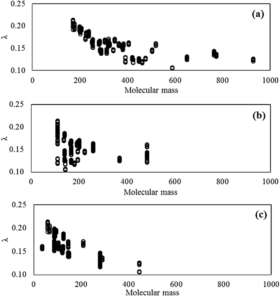
Thermal conductivity as a function of the molecular mass of all ionic liquids used in this study. (a) Total mass distribution, (b) cation distribution, and (c) anion distribution.

Additionally, molecular mass M and molecular structures, represented by the number of well-defined groups forming the molecule, were provided as input parameters in order to characterize the different molecules of ILs. A leave-25%-out cross-validation method was used to estimate the predictive capabilities of the proposed method for entrances such as temperature T, pressure P, molecular mass M, and 28 structural groups. Thus, the whole dataset was divided into a training set with 300 experimental data points, and a prediction set with 100 experimental data points. Table S1 shows the values of experimental thermal conductivity considered in this study (see Supplementary data). Training and prediction sets were selected considering that molecules were decomposed into fragments and all fragments were present with adequate frequency in the training dataset for structural groups. The value associated with the structural group was defined as 0 when the group does not appear in the substance, and as k, when the group appeared k-times in the substance [26]. Table 1 shows all 31 input parameters considered in this study, and contains minimum and maximum input values, and the number of input occurrences in the datasets.

No.	Input	X^min	X^max	No. occurrence
Training set	Prediction set	Total set
1	T	273.15	390.00	300	100	400
2	P	100	20000	300	100	400
3	M	66.43	515.13	300	100	400
4	Imidazolium⁽⁺⁾	0	1	199	42	241
5	Pyridinium⁽⁺⁾	0	1	18	9	27
6	Pyrrolidinium⁽⁺⁾	0	1	7	9	16
7	Ammonium⁽⁺⁾	0	1	30	7	37
8	Phosphonium⁽⁺⁾	0	1	46	33	79
9	–H⁽⁺⁾	0	1	217	41	258
10	– ${CH}_{3}$ ⁽⁺⁾	1	4	300	100	400
11	–CH₂–⁽⁺⁾	1	28	300	100	400
12	– ${CH}_{3}$ ⁽⁻⁾	0	4	74	5	79
13	–CH₂–⁽⁻⁾	0	10	56	14	70
14	>CH–⁽⁻⁾ [–CH–]⁽⁻⁾	0	2	51	12	63
15	>C<⁽⁻⁾ [>C–]⁽⁻⁾	0	1	23	5	28
16	–COO–⁽⁻⁾	0	1	9	0	9
17	–COOH⁽⁻⁾	0	1	42	12	54
18	–OH⁽⁻⁾	0	1	30	7	37
19	–O–⁽⁻⁾ [–O]⁽⁻⁾	0	2	65	14	79
20	O⁽⁻⁾	0	1	9	0	9
21	–CN⁽⁻⁾	0	3	9	9	18
22	>N–⁽⁻⁾	0	1	64	49	113
23	– ${NH}_{2}$ ⁽⁻⁾	0	2	42	26	68
24	–SO₂–⁽⁻⁾	0	2	111	54	165
25	–SH⁽⁻⁾	0	1	7	0	7
26	– ${CF}_{3}$ ⁽⁻⁾	0	3	94	40	134
27	–CF₂–⁽⁻⁾	0	3	16	0	16
28	–F⁽⁻⁾	0	6	104	25	129
29	–Cl⁽⁻⁾	0	1	7	0	7
30	–P⁽⁻⁾	0	1	59	16	75
31	–B⁽⁻⁾	0	1	63	9	72

Subsequently, these input parameters were normalized using the following equation [11]:

x_{i} = (X_{i} - X_{i}^{min}) \frac{2}{X_{i}^{max} - X_{i}^{min}} - 1

(3)

where X_i is the input variable i, and X_i^min and X_i^max are the smallest and largest values of the data, respectively. Thus, the net inputs (N) are calculated for the hidden neurons coming from the input neurons as shown in Eq. (1), and then a GA is used to obtain the optimum weights for the feed-forward ANN.

The step-by-step for optimum weights calculation using GA is described as follows:

1) Initial weights in the ANN are randomly generated (initial population). M-chromosomes are generated randomly in order to serve as the initial population. Each chromosome represents all initial weights and biases in the ANN, which are optimized by the GA.
2) Chromosome fitness is evaluated based on the ANN performance. In this case, the fitness function is defined as the root mean square error (RMSE).
3) Fitness function value of each individual in the population is evaluated. The lower the RMSE, the higher the probability for chromosomes to be passed down to the next generation. The best individual chromosomes are selected for mating. The selection is repeated until the number of individuals in the mating pool is the same as the number of individuals in the population [26].
4) Two individuals are selected randomly from the mating pool as the parent, and random gene selection is used as a crossover point [26]. The transfer of the parent genes to the right of the crossover point generates two new individuals, ending of the single-point crossover [27].
5) A mutation operator is applied in order to maintain diversity within the population. Since the initial weights of the ANN could take any values between zero and one, the mutation is conducted by switching random genes. The approximate optimum solutions can be found quickly in order to set up the mutation rate as a parameter to control mutation probability. The mutation rate is a real number between 0 and 1 [28].
6) Finally, the best chromosome with the minimum RMSE is chosen and set as the initial weights for the next period in the ANN. The process is repeated until the convergence toward a population of individuals encoding the set of weights that keep the error at a desired level occurs.

Fig. 2 shows a block diagram of the ANN+GA developed in this study. The full methodology was programmed in C++. In a GA, the number of individuals, the crossover operator, the crossover probability, the mutation operator, and the mutation probability summarize the parameters for synchronizing their application in a given problem. An exhaustive trial-and-error procedure was applied for tuning GA parameters. Table 2 shows the selected parameters for the ANN+GA algorithm.

Fig. 2
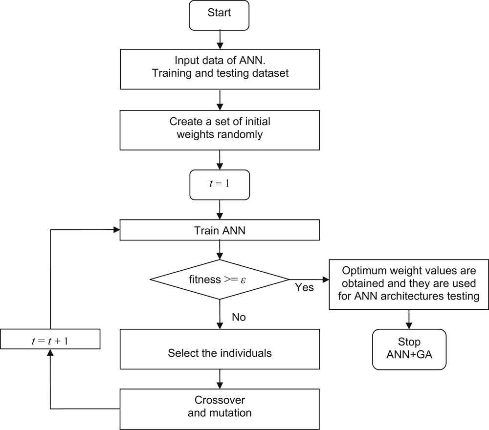
Flow diagram for training of the ANN using GA.

Section	Parameter	Value
ANN	NN-type	feed-forward
No. hidden layers	1
Transfer function (hidden)	tansig
Transfer function (output)	linear
No. iterations	1500
Normalization range	[−1, 1]
Weight range	[−35, 35]
Minimum error	1e−4
GA	No. individuals	100
Crossover operator	two point
Crossover probability	0.8
Mutation operator	binary
Mutation probability	0.02
Objective function	RMSE

Using the above methodology, several network architectures were tested to select the most accurate topology. The most basic architecture usually used for this type of application involves a neural network consisting of three layers [29]. The number of hidden neurons should be sufficient for ensuring an adequate representation of the information in the data used for training the network [2]. There is no specific approach for determining the number of neurons of the hidden layer (NHL), but many alternative combinations are possible. Therefore, the optimum number of neurons was determined by systematically adding neurons and evaluating the RMSE of the sets during the learning process [29]. Fig. 3 shows the RMSE found when correlating λ(T,P) as a function of the number of neurons in the hidden layer. As observed in this figure, the optimum number of neurons in the hidden layer is between 4 and 6. The network giving the lowest deviation during training was the one with 31 parameters in the input layer, 5 neurons in the hidden layer, and one neuron in the output layer. The RMSEs of this architecture were 0.00199 during training, and 0.00197 during prediction, respectively.

Fig. 3
Root mean square error (RMSE) found in correlating the λ(T,P) of ILs as a function of the number of neurons in the hidden layer (NHL) using ANN+GA. Training step (●) and prediction step (◊).

4 Results and discussion

Once the best architecture was determined, the optimum weights required to carry out the estimate λ(T,P) of ILs were obtained. Table 3 shows the optimum weights for the ANN+GA 31-5-1.

Input	W_ij	1	2	3	4	5
T	1	−0.78316	0.00703	−0.17960	0.26168	0.04082
P	2	0.67404	0.01776	−0.28596	−0.08177	0.02026
M	3	0.49567	−0.42633	−0.33646	0.51141	−1.92883
Imidazolium⁽⁺⁾	4	−0.16750	−1.16420	2.85627	1.42302	0.53367
Pyridinium⁽⁺⁾	5	2.23931	0.57646	6.45933	−0.86621	0.11607
Pyrrolidinium⁽⁺⁾	6	−0.75567	1.19110	−0.72874	−1.65053	−0.62319
Ammonium⁽⁺⁾	7	−0.43186	0.06006	0.10105	−1.37138	−0.54707
Phosphonium⁽⁺⁾	8	−0.81134	−0.47999	−9.26492	1.61749	2.96438
–H⁽⁺⁾	9	−0.93286	−0.95518	9.89140	0.15419	0.19737
– ${CH}_{3}$ ⁽⁺⁾	10	−0.76023	−0.64633	−8.34596	0.68890	1.17553
–CH₂–⁽⁺⁾	11	0.72921	−2.01568	34.54003	0.97577	−2.75101
– ${CH}_{3}$ ⁽⁻⁾	12	−0.35701	0.05285	−0.08003	0.55303	0.21510
–CH₂–⁽⁻⁾	13	1.66628	−0.28268	−0.15251	−0.10097	−0.15836
>CH–⁽⁻⁾ [–CH–]⁽⁻⁾	14	−0.32900	−0.32869	0.25780	−0.75351	−0.34744
>C<⁽⁻⁾ [>C–]⁽⁻⁾	15	−0.36681	−0.15418	−0.07819	−0.26981	−0.01303
–COO–⁽⁻⁾	16	0.80487	1.64832	−0.74100	−1.34253	0.33933
–COOH⁽⁻⁾	17	0.34297	−0.55203	−0.21594	0.93211	0.86835
–OH⁽⁻⁾	18	−0.04608	0.00796	0.79831	0.09337	−0.41559
–O–⁽⁻⁾ [–O]⁽⁻⁾	19	−0.91670	0.79096	0.74844	0.23056	2.02816
O⁽⁻⁾	20	−0.27203	−0.11996	1.04748	−1.99322	−0.72868
–CN⁽⁻⁾	21	0.68336	1.58632	−0.89114	−1.31813	0.43514
>N–⁽⁻⁾	22	−0.18281	−1.47621	−1.27767	2.78803	1.16030
– ${NH}_{2}$ ⁽⁻⁾	23	−1.18164	0.24742	−0.03550	0.13463	−0.52892
–SO₂–⁽⁻⁾	24	−0.31328	−2.36592	−0.25911	0.78516	−1.13372
–SH⁽⁻⁾	25	−0.01235	0.03879	−0.27630	0.87636	−0.11776
– ${CF}_{3}$ ⁽⁻⁾	26	−1.00636	−1.26141	−1.99734	0.77169	0.57938
–CF₂–⁽⁻⁾	27	−0.36883	1.13458	−2.08071	−0.36091	−1.08332
–F⁽⁻⁾	28	1.22737	−0.57960	0.29477	1.41748	1.66512
–Cl⁽⁻⁾	29	1.06402	−0.38947	0.04274	−0.52829	−0.41591
–P⁽⁻⁾	30	−0.60428	0.08309	2.65385	−0.69970	−0.41548
–B⁽⁻⁾	31	−0.38003	−0.20115	−2.50992	−0.15801	−0.06608
	W_0j	1.52286	−0.41596	0.31931	−0.68584	−2.44430
	W_nj	0.29242	−13.79025	0.20755	−13.64070	7.61938
	W_n0	7.26828

The accuracy of the chosen network was verified between the calculated values of λ and the experimental data from the literature, by using the average relative absolute deviation for each data point (|%Δλ|) and for the total set (AARD). These deviations were calculated as follows:

| % Δ λ | = | \frac{λ^{calc} - λ^{exp}}{λ^{exp}} | \cdot 100

(4)

AARD = \frac{100}{N_{data}} \sum_{i = 1}^{N} {| \frac{λ^{calc} - λ^{exp}}{λ^{exp}} |}_{i}

(5)

Table S1 shows the results obtained for the correlation set and prediction set, respectively (see, Supplementary data). Table 4 shows the results obtained from the proposed GCM for all different types of ILs; it shows the following ranges of AARD in the prediction of λ(T,P): ammonium < pyridinium < imidazolium < phosphonium < 1%, and pyrrolidinium < 3%. All IL-types presented a maximum error lower than 4%, and all the correlation coefficients R² are greater than 0.9. Table 5 shows a summary of the deviations of all ILs using the proposed ANN+GA method. The results showed that the ANN+GA can provide an accurate estimation of the thermal conductivity of several ILs: AARD lower than 0.91% for the 300 data points used in the training set, and an AARD lower than 0.84% for the other 100 data points used in the prediction set. The AARD is a little higher than 0.8% for all datasets (400 data points of several ILs), and the deviation is lower than 5% for all data points of the database.

IL class	N_data	Δλ (W m⁻¹ K⁻¹)	ΔT (K)	ΔP (kPa)	AARD	\|%Δλ\|_min	\|%Δλ\|_max	R²
Training set
Imidazolium	199	0.12–0.22	273−390	100−20000	1.27	0.00	4.96	0.9961
Ammonium	30	0.12–0.17	273−353	101	0.21	0.00	0.98	0.9997
Pyridinium	18	0.16–0.17	294−334	100−20000	0.24	0.00	0.55	0.9934
Phosphonium	46	0.12–0.16	282−355	101	0.19	0.00	0.64	0.9997
Pyrrolidinium	7	0.11–0.13	293−353	101	0.22	0.03	0.43	0.9937
Prediction set
Imidazolium	42	0.13–0.21	273−390	100−20000	0.68	0.03	2.22	0.9987
Ammonium	7	0.16–0.17	298−353	101	0.09	0.00	0.16	0.9981
Pyridinium	9	0.16–0.17	294−334	100−20000	0.38	0.00	1.08	0.9896
Phosphonium	33	0.13–0.16	286−353	101	0.85	0.00	3.42	0.9878
Pyrrolidinium	9	0.12–0.13	293−333	101	2.67	1.79	3.53	0.9288

Statistics	Correlation set	Prediction set	Total set
N_data	300	100	400
AARD	0.91	0.84	0.89
\|%Δλ\|_min	0.00	0.00	0.00
\|%Δλ\|_max	4.96	3.53	4.96
\|%Δλ\|<5%	300	100	400
\|%Δλ\|>5%	0	0	0
R²	0.9969	0.9963	0.9967

Fig. 4 shows a comparison between experimental (solid line) and calculated (dots) values by the proposed ANN+GA method to estimate λ(T,P). This figure shows a comparison between correlated and experimental values of thermal conductivity. For the training set, the correlation coefficient R² was 0.9969, and the curve slope (m) was 0.9947 (expected to be 1.0). Also, the figure shows a comparison for the prediction set between calculated and experimental values of λ. In this case, the correlation coefficient R² is 0.9963 and m (also expected to be 1.0) is 0.9926. For the total set, the correlation coefficient R² is 0.9967 and m is 0.9945. This figure ratifies the discussion presented above.

Fig. 4
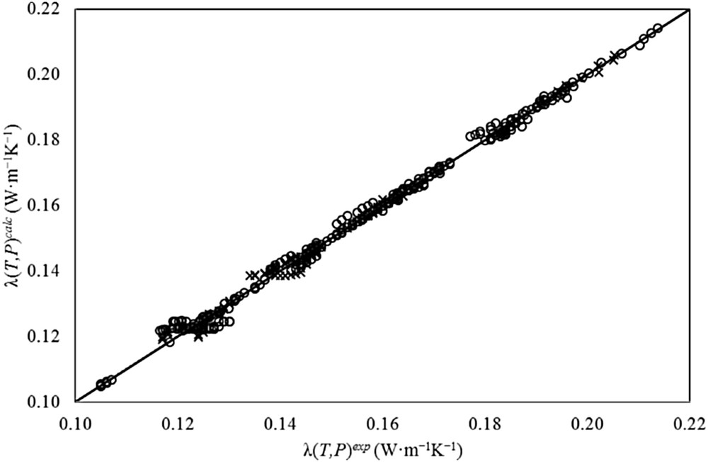
Accuracy in the estimation of thermal conductivity of ILs with the proposed ANN+GA method. (○) training set, and (×) prediction set.

Note that for the estimation of λ(T,P = 101.325 kappa), the prediction set presents a very low deviation (AARD = 0.88%) with an |%Δλ|_max of 3.53%. In particular, the dataset of 1-butyl-1-methylpyrrolidinium bis[(trifluoromethyl)sulfonyl]imide [20] showed a highest AARD of 2.92%. In addition, the prediction set also showed a very low AARD of 0.66% with a |%Δλ|_max of 2.22% for the estimation of the thermal conductivity at different temperatures and pressures λ(T,P). In this case, the prediction set presents an AARD of 0.40% for pressures higher than the atmospheric pressure (P > 101.325 kappa).

Recently a number of methods have been proposed for the estimation of thermal conductivity of ILs [30] (see, the Introduction section). It is worth pointing out that all these methods obtained their results from different databases with different correlation and prediction sets (or training and prediction sets), and based on different methodologies and the results cannot be compared directly with one another. However, a comparison can be made for the selected datasets of common ILs for all methods. Table 6 shows a comparison between the proposed neural network method for the λ estimation of ILs and other methods reported in the literature such as group contribution methods (GCM), generalized correlations, and quantitative structure–property relationships (QSPR). This table contains 20 datasets of ILs at atmospheric pressure and several temperatures. Only four methods can be completely compared based on these results. Albert−Müller's GCM [8] showed an AARD of 2.19, Wu's method [9] presented an AARD of 1.89, Lazzús's QSPR model [30] resulted in an AARD of 2.09, and the proposed neural network method showed an AARD of 1.35. On the one hand, Gardas–Coutinho's GCM [7] does not perform for any ILs due to the group division principle, and it cannot be extended to others ILs [30]. On the other hand, Wu's method [9] and Shojaee's method [3] depend on the knowledge of other properties of ILs. Therefore, the proposed neural network method presented better accuracy and more advantages than other methods to predict λ of ILs at atmospheric pressure and different temperatures.

Ionic liquid	ΔT (K)	N_data	Gardas−Coutinho GCM [7] AARD	Albert−Müller GCM [8] AARD	Wu et al. Correlation [9] AARD	Shojaee et al. Correlation [3] AARD	Lazzús QSPR [30] AARD	This work ANN+GA	Ref.
[C2mim][NTf2]	273.15–353.15	9	6.41	4.02	5.84	6.54	3.69	3.83	[6]
[C2mim][EtSO4]	293.00–353.00	7	0.15	2.00	1.30	9.34	3.50	0.87	[20]
273.15–353.15	9	2.53	1.10	11.16	0.89	0.74	[6]
[C2mim][CH3COO]	273.17–353.15	9	–	0.85	0.86	–	3.32	0.25	[6]
[C2mim][DCA]	273.17–353.15	9	–	1.76	0.58	14.72	0.80	0.31	[6]
[C2mim][C(CN)3]	273.17–353.15	9	–	0.33	0.74	–	1.52	0.27	[6]
[C4mim][OTf]	293.00–353.00	7	0.15	1.71	0.37	1.92	0.55	1.68	[20]
293.00–353.00	7	3.51	3.09	3.82	3.00	1.74	[21]
[C4mim][NTf2]	293.00–353.00	7	1.26	2.65	1.00	3.29	3.21	2.38	[20]
[C4mim][PF6]	293.00–353.00	7	0.98	0.88	1.55	2.40	0.96	0.26	[21]
294.90–335.10	3	0.69	1.40	–	1.01	0.34	[5]
[C6mim][NTf2]	293.00–353.00	7	1.40	1.69	1.97	3.66	2.65	3.03	[20]
273.15–353.15	9	5.26	1.88	5.34	1.00	0.78	[6]
[C6mim][BF4]	293.00–353.00	7	23.09	4.55	1.20	0.76	0.72	2.03	[21]
[C6mim][PF6]	293.00–353.00	7	4.32	2.07	1.51	2.27	4.00	1.21	[21]
294.10–335.20	3	0.95	1.78	–	1.35	0.95	[5]
[C8mim][PF6]	295.10–335.20	3	1.20	2.07	3.02	–	3.15	0.49	[5]
[C8mim][NTf2]	293.00–353.00	7	1.09	3.41	3.01	–	1.01	0.46	[20]
[C4mpyrr][NTf2]	293.00–323.00	4	0.19	2.65	0.77	6.05	2.98	2.92	[20]
293.00–333.00	5	5.84	4.76	10.91	2.52	2.47	[21]
AARD	3.47	2.19	1.89	5.87	2.09	1.35

In other comparison, using Shojaee's method [3] at different pressures (100−20000 kappa) resulted in an AARD of 3.47% for three ILs, while the proposed neural network method showed an AARD of 0.64%. Table 7 shows the ILs and ranges of temperatures and pressures used in this comparison. Table 7 clearly shows that the proposed neural network method offered better accuracy and more advantages in the λ estimation of ILs at several temperatures and pressures only by knowing the molecular structure of IL.

Ionic liquid	ΔT (K)	ΔP (kPa)	N_data	Shojaee et al. Correlation [3] AARD	This work ANN+GA AARD	Ref.
[C₄mim][PF₆]	294.90–335.10	100–20000	9	3.16	0.47	[5]
[C₆mim][PF₆]	294.10–335.20	100–20000	9	2.97	0.95	[5]
[C₈mim][PF₆]	294.10–335.20	100–20000	9	4.29	0.49	[5]
AARD	3.47	0.64

In addition to these results, a comparison was made with a neural network with standard back-propagation (BPNN), and similar architecture (31-5-1) and database. The BPNN showed an AARD of 2.5%, and a |%Δλ|_max higher than 15%. Fig. 5 shows a |%Δλ| found during the prediction of thermal conductivity of ILs using the BPNN versus a |%Δλ| obtained using the proposed ANN+GA method. In other applications relative to BPNN, Hezave et al. [12] presented a neural network model to predict thermal conductivity of ionic liquids. In Hezave's neural network model a total of 209 data points from 21 different ionic liquids were used to train and test the BPNN, and the optimum architecture was determined to be 4-13-1, with input parameters such as temperature T, pressure P, molecular weight MW, and melting point temperature T_m. A considerable disadvantage of Hezave's neural network model is the use of melting point temperature of ILs. Note that, for organic compounds, Pérez Ponce et al. [31] showed an AARD higher than 7.5% for several methods reported during years 1987–2006; additionally, they presented an AARD for three commercial softwares for predicting T_m with an AARD higher than 12% and maximum deviations higher than 45%. For ILs, Huo et al. [32] presented a group contribution method (GCM) for estimating the melting point of imidazolium-ILs with an AARD of 5.9% and maximum deviations higher than 32%. Coutinho et al. [33] presented a critical review on predictive methods for the estimation of thermophysical properties of ILs, with R² from 0.6 to 0.9 for the prediction of T_m. Thus, the reliability of the input data is never established, making interpretation of deviations between the Hezave's neural network model and experimental data of thermal conductivity of ILs impossible to be made. In contrast, low deviations from the proposed ANN+GA method (an AARD a little higher than 0.8% and a |%Δλ|_max below than 5%) indicate that it can estimate λ(T,P) of ILs with low deviations and can be relied on an accuracy of 99%. All these results represent a big increase in accuracy for predicting this important property, and show that the application of the proposed ANN+GA method was crucial. An important observation that is worth pointing out is the influential effects of the structural groups in the correlation and prediction of the thermal conductivity. Considering that the big differences in the chemical structure and physical properties of the ILs used in the study place additional difficulties that the proposed ANN+GA method was able to handle.

Fig. 5
Deviations found in the prediction of λ(T,P) of ILs using ANN+GA (○) and BPNN (Ж).

The incorporation of a GA for the optimization of the neural network weights has positive effects on architecture reducing the number of neurons in the hidden layer while controlling the selection of network connection weightings in a wide numeric range (see, Table 2). Note that, traditional optimization techniques such as the back-propagation learning algorithm can also determine the number of network parameters, such as network connection weightings; however, traditional optimization techniques are not able to control the network parameter optimizations. In contrast, the GA was able to solve this problem.

5 Conclusions

In this study, the thermal conductivity of several ILs at different temperatures and pressures was correlated and estimated using an artificial neural network optimized with a genetic algorithm in order to update the weights of the network.

Based on the results and discussion presented in this study, the following conclusions are obtained: (i) the great differences in the chemical structure, and the physical properties of the ionic liquids considered in the study impose additional difficulties to the problems that the proposed ANN+GA method has been able to handle; (ii) the results show that the ANN+GA method can estimate the thermal conductivity of ionic liquids at different temperatures and pressures with low deviations. The consistency of the method has been checked using experimental values of thermal conductivity and comparing them with the calculated values by the proposed method; (iii) the values calculated using the proposed model are believed to be accurate enough for engineering calculations, for generalized correlations and for equations of state methods, among other uses; and (iv) the incorporation of a GA for the optimization of the neural network weights has positive effects on architecture reducing the number of neurons in the hidden layer while controlling the selection of network connection weightings in a wide numeric range.

Acknowledgements

The author thanks the Direction of Research of the University of La Serena (DIULS), through the research project PT13144. Special thanks go to the Department of Physics of the University of La Serena (DFULS) for the special support that made possible the preparation of this paper.

Bibliographie

[1] H. Ohno Electrochemical Aspects of Ionic Liquids, John Wiley & Sons, New Jersey, 2005

[2] J.A. Lazzús Int. J. Thermophys., 30 (2009), pp. 883-909

[3] S.A. Shojaee; S. Farzam; A.Z. Hezave; M. Lashkarbolooki; S. Ayatollahi Fluid Phase Equilib., 354 (2013), pp. 199-206

[4] C. Frez; G.J. Diebold; C.D. Tran; S. Yu J. Chem. Eng. Data, 51 (2006), pp. 1250-1255

[5] D. Tomida; S. Kenmochi; T. Tsukada; K. Qiao; C. Yokoyama Int. J. Thermophys., 28 (2007), pp. 1147-1160

[6] A.P. Fröba; M.H. Rausch; K. Krzeminski; D. Assenbaum; P. Wasserscheid; A. Leipertz Int. J. Thermophys., 31 (2010), pp. 2059-2077

[7] R.L. Gardas; J.A.P. Coutinho AIChE J., 55 (2009), pp. 1274-1290

[8] J. Albert; K. Müller Ind. Eng. Chem. Res., 53 (2014), pp. 17522-17526

[9] K.-J. Wu; C.-X. Zhao; C.-H. He Fluid Phase Equilib., 339 (2013), pp. 10-14

[10] J.O. Valderrama; W.W. Sanga; J.A. Lazzús Ind. Eng. Chem. Res., 47 (2008), pp. 1318-1330

[11] M.T. Hagan; H.B. Demuth; M. Beal Neural Network Design, PWS Publishing Company, Boston, USA, 1996

[12] A.Z. Hezave; S. Raeissi; M. Lashkarbolooki Ind. Eng. Chem. Res., 51 (2012), pp. 9886-9893

[13] J. Holland Adaptation in Natural and Artificial Systems, University of Michigan Press, Michigan, USA, 1975

[14] L. Davis Handbook of Genetic Algorithms, Van Nostrand Reinhold, New York, USA, 1991

[15] J.A. Lazzús; M. Rivera Rev. Mex. Fís., 59 (2013), pp. 577-583

[16] Q. Dong; C.D. Muzny; A. Kazakov; V. Diky; J.W. Magee; J.A. Widegren; R.D. Chirico; K.N. Marsh; M. Frenkel J. Chem. Eng. Data, 52 (2007), pp. 1151-1159

[17] Q.-L. Chen; K.-J. Wu; C.-H. He J. Chem. Eng. Data, 58 (2013), pp. 2058-2064

[18] A.G.M. Ferreira; P.N. Simoes; A.F. Ferreira; M.A. Fonseca; M.S.A. Oliveira; A.S.M. Trino J. Chem. Thermodyn., 64 (2013), pp. 80-92

[19] R.L. Gardas; R. Ge; P. Goodrich; C. Hardacre; A. Hussain; D.W. Rooney J. Chem. Eng. Data, 55 (2010), pp. 1505-1515

[20] R. Ge; C. Hardacre; P. Nancarrow; D.W. Rooney J. Chem. Eng. Data, 52 (2007), pp. 1819-1823

[21] C.A. Nieto de Castro; M.J.V. Lourenco; A.P.C. Ribeiro; E. Langa; S.I.C. Vieira J. Chem. Eng. Data, 55 (2010), pp. 653-661

[22] D. Tomida; S. Kenmochi; K. Qiao; T. Tsukada; C. Yokoyama Fluid Phase Equilib., 340 (2013), pp. 31-36

[23] D. Tomida; S. Kenmochi; T. Tsukada; K. Qiao; Q. Bao; C. Yokoyama Int. J. Thermophys., 33 (2012), pp. 959-969

[24] M.E. Van Valkenburg; R.L. Vaughn; M. Williams; J.S. Wilkes Thermochim. Acta, 425 (2005), pp. 181-188

[25] J.A. Lazzús Fluid Phase Equilib., 313 (2012), pp. 1-6

[26] Z.-G. Che; T.-A. Chiang; Z.-H. Che Int. J. Innovative Comput., 7 (2011), pp. 5839-5850

[27] A. Meng; L. Ye; D. Roy; P. Padilla Comput. Educ., 49 (2007), pp. 1205-1223

[28] E. Eiben; R. Hinterding; Z. Michalewicz IEEE Trans. Evolut. Comput., 3 (1999), pp. 124-141

[29] J.A. Lazzús; I. Salfate; S. Montecinos Neural Netw. World, 24 (2014), pp. 601-617

[30] J.A. Lazzús; G. Pulgar-Villarroel J. Mol. Liq., 211 (2015), pp. 981-985

[31] A.A. Pérez Ponce; I. Salfate; G. Pulgar-Villarroel; L. Palma-Chilla; J.A. Lazzús J. Eng. Thermophys., 22 (2013), pp. 226-235

[32] Y. Huo; S. Xia; Y. Zhang; P. Ma Ind. Eng. Chem. Res., 48 (2009), pp. 2212-2217

[33] J.A.P. Coutinho; P.J. Carvalho; N.M.C. Oliveira RSC Adv., 2 (2012), pp. 7322-7346

Commentaires - Politique

Ces articles pourraient vous intéresser

Semi-empirical correlation of solid solute solubility in supercritical carbon dioxide: Comparative study and proposition of a novel density-based model

Aicha Belghait; Cherif Si-Moussa; Maamar Laidi; ...

C. R. Chim (2018)

Novel density-based model for the correlation of solid drugs solubility in supercritical carbon dioxide

Cherif Si-Moussa; Aicha Belghait; Latifa Khaouane; ...

C. R. Chim (2017)

Glass transition temperature of ionic liquids using molecular descriptors and artificial neural networks

José O. Valderrama; Richard A. Campusano; Roberto E. Rojas

C. R. Chim (2017)