

1 Introduction
The phenomenon of the spin transition is relatively recent. This phenomenon was first mentioned by Cambi and Szegö [1] when they noticed what they called anomalous behavior in the magnetic behavior of their compounds based on Fe(III) tris(dithiocarbamate). But it was not until 1956 when Ballhausen and Liehr introduced the spin equilibrium notion of certain tetracoordinated Ni(II) compounds [2]. This conversion of spin states was verified in 1961 in a cobalt compound by studying the variation in the magnetic moment as a function of temperature [3]. Concerning Fe(II), which is by far the most used by scientists to obtain spin crossover (SCO) materials, the first compound published was the [Fe(phen)2(SCN)2], where phen is the 1,10-phenanthroline. This compound shows an abrupt spin transition at 170 K with a small hysteresis loop [4].
Today, this phenomenon called spin conversion, spin transition or, more frequently, SCO is well understood essentially because it has been the object of in-depth multidisciplinary research drive by chemists, physicists, spectroscopists, crystallographers, theoreticians, and material scientists in general. It remains one of the most spectacular forms of a switchable material with great future prospects [5–10].
Here, we should mention that along this review we have to introduce certain concepts that probably have been carefully considered previously in this special issue, nonetheless these concepts should be fresh in the mind for a better understanding of this work.
Spin-transition materials are observed in coordination complexes of first-row transition metal ions with d4 to d7 electronic configuration. Although this property is not homogeneously distributed among the ions, it can be observed mainly in Fe(II), Fe(III), and Co(II), and also in Mn(II), Mn(III), Cr(II), Cr(III), and Ni(II) ions [11]. Nevertheless, it is clearly iron(II) in octahedral symmetry, which exhibits the greatest proportion of SCO complexes.
Therefore, a good starting point to explain the spin transition phenomenon is the use of crystal field theory (CFT) [12]. CFT is an electrostatic model that considers the metal to be positively charged whereas the ligands are negatively charged. CFT describes the electron distribution in the d or f orbitals of a metal ion under different symmetries and explains the interactions between the metal and ligands in coordination complexes with transition metals. This implies an electrostatic attraction between the pairs of electrons of the ligands and the positively charged metal ion. This simple model supposes a free and gaseous metal ion and involves the ligands as point charges with no interaction between the metal and ligand orbitals. First, the approach of the ligand electrons to the metal ion modifies the energy of metal ion d orbitals. Depending on the geometry of the complex, the metal orbitals along the bonding directions with the ligands will increase their energy, whereas the electrons located between them decrease their energy (see Fig. 1).
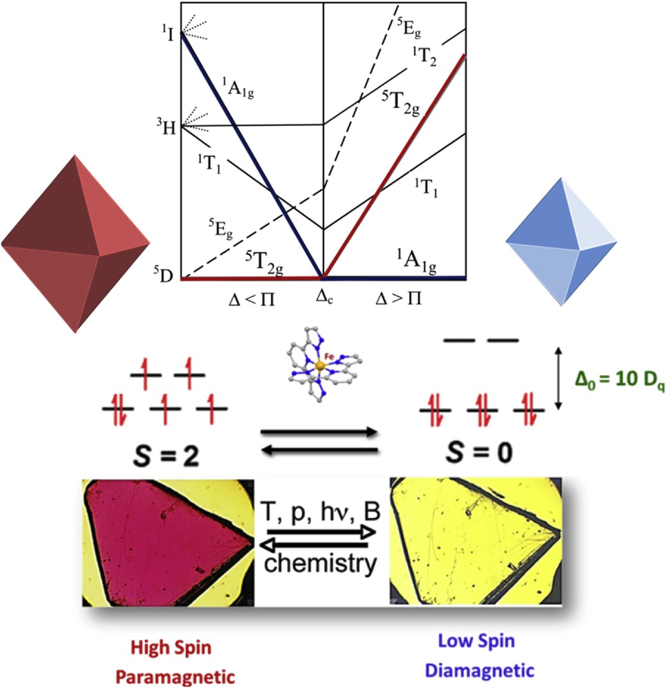
Representation of the two spin states of an ion with six d electrons. (Top) A simplified Tanabe–Sugano diagram showing the energy dependence of the HS and LS states as a function of the ligand field. (Middle) An electronic array in the HS and LS states. (Bottom) An illustration of the color modification in an SCO sample.
For octahedral complexes and more specifically for Fe(II) complexes, the six ligands are distributed along the Cartesian axes. As a result of the presence of these negative charges, the dx2−y2 and dz2 orbital energies will be considerably higher than the others, with the energy difference defined as 10 Dq [13]. When 10 Dq is lower than the electron spin pairing energy (Π), in a weak ligand field configuration, the electrons in the complex follow Hund's rule of maximum multiplicity. The number of unpaired electrons is maximized and the electrons occupy also the high energy orbitals, being the total spin, S = 2 for the Fe(II). In this case, the paramagnetic state is called high spin (HS) (Fig. 1). On the other hand, strong ligand fields generate systems where 10 Dq is larger than Π, favoring electron pairing because the low energy orbitals are preferably occupied. This situation generates a total spin, S = 0 for Fe(II). This diamagnetic state is named low spin (LS).
Occasionally, the balance between these two states is so delicate that modulation of an external parameter is sufficient to reversibly switch between them. This external perturbation provokes the so-called SCO. Temperature variation is the most common method to switch between the spin states, although it can also be achieved through irradiation with light [14–17], pressure [18], an external magnetic field [19], or the inclusion of small molecules into the material [20–24]. The marked difference in physical properties between the two different spin states means that a variety of experimental techniques can be used to detect and follow the progress of a spin transition.
2 Basic principles of the three macroscopic physical techniques used to study the SCO phenomenon
As mentioned, the SCO is accompanied by drastic changes in various structural and electronic properties. For instance, the magnetic properties change dramatically with the SCO phenomenon. For an iron(II) metal ion with no unpaired electron in the LS state, the compound is diamagnetic or weakly paramagnetic but with four unpaired electrons in the HS the compound is strongly paramagnetic. This drastic difference is easily monitored by measuring the magnetic susceptibility.
Therefore, the optical spectrum in the UV–vis region differs drastically for the two spin states and is therefore well suited to follow the spin transition qualitatively and quantitatively. Finally, calorimetric measurements are used to determine the effective enthalpy and entropy changes accompanying the spin transition. The following section will provide a general description of how magnetic, optical, and calorimetric methods can be used to detect the SCO phenomena.
2.1 Magnetic methods
Clearly, the most important property in magnetochemistry is to measure the magnetization (M) of a sample. As per Prof. J. Ribas-Gispert [25], this can be defined as “what happens inside the sample when a homogeneous magnetic field is applied to the sample”. This question is, of course, of paramount relevance for the SCO compounds.
When the sample is exposed to a homogeneous external magnetic field, H, a magnetization M is induced in the sample. In the case that the applied field is not too strong, M in the sample may be expressed as the magnetic susceptibility χ, defined as follows [13,25]:
| (1) |
This measured susceptibility is the algebraic sum of two contributions that are associated with different phenomena:
| (2) |
| (3) |
The magnetic susceptibility can be expressed with three different expressions related to volume Χv, mass Χg, or molecular weight Χm with the last one being the most commonly used. Because the SCO occurs generally in mononuclear compounds, we can use a simplification of the Van Vleck formula [26]:
| (4) |
In Fig. 2, the χmT versus T plot of a core–shell SCO particles that have been synthesized from a coordination polymer with formula [Fe(trz)(H-trz)2](BF4) (where H-trz = 1,2,4-triazole and trz = 1,2,4-triazolato) is shown. The spin transition may then be followed by varying the temperature of the sample and measuring the change in the magnetic susceptibility, which has been transformed into the HS evolution fraction [28].
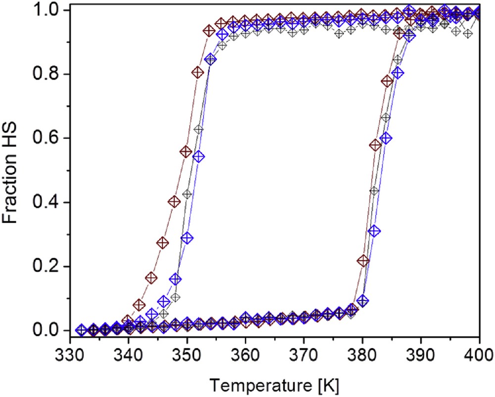
Temperature dependence of the HS fraction for the nanocomposite core–shell SCO particles synthesized from the coordination polymer [Fe(trz)(H-trz)2](BF4) (H-trz = 1,2,4-triazole and trz = 1,2,4-triazolato) on heating and cooling (second thermal cycle) [28].
After this theoretical consideration an important question arises: how can the magnetization be measured? In fact there are many magnetometers capable of measuring the magnetization of a sample, for example, the faraday torque balance [29], the vibrating sample magnetometer [30], and, likely the most popular, the superconducting quantum interference device (SQUID) [31].
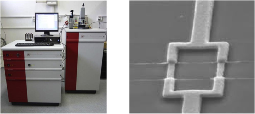
In more detail, SQUID (Fig. 3, left) is an electronic system that uses a superconducting ring into which one or two small insulating layers have been inserted (Fig. 3, right). This device is based on the Josephson effect in a superconductor–insulator–superconductor sandwich, where flux quantization in the ring makes it ultrasensitive to any magnetic field. Commercial SQUID magnetometers offer a high sensitivity (5 × 10⁻⁸ emu) and are easy to use; besides, they can access a large range of temperatures (higher than 500 K and lower than 1 K).
The SQUID measure complicated physical phenomena that occur in the sample when a magnetic field is applied but in the end these processes are expressed in terms of magnetization.
2.2 Optical methods
Color is a well-known property of transition metals. Colors are produced as parts of the visible spectrum are absorbed by a material due to electron transitions between its energy levels, the color we see in coordination compounds being due to absorption by electrons in the d orbitals. As mentioned above, SCO provokes a drastic split within the d orbitals into two different electronic states (HS and LS) with a difference in energy. Therefore, an important color change may occur while passing from one state to the other. Thus, monitoring the color of the sample can afford important information about the nature of the spin transition, including how the sample will behave in both solid and solution states.
We shall come back to the Tanabe–Sugano diagram (see Fig. 1, top) to explain in more detail how this electronic rearrangement works. For an octahedral d6 complex we can see that in the region of the left of the crossover point, the term 5T2 is the ground state and only one spin-allowed transition, 5T2 → 5Eg can be expected. To the right of this point, the 1A1 is the ground state term and two spin-allowed transitions, 1A1 → 1T1 and 1A1 → 1T2 are then predicted to appear in the UV–vis [32].
The same process is exactly what happens in solution. We observe a relatively weak quintet–quintet band of the colorless crystal in the HS state (Fig. 4, left) and more intense single–singlet transitions in the LS (Fig. 4, right).
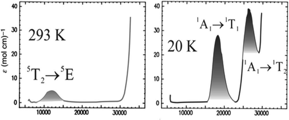
Single crystal UV–vis absorption spectra for [Fe(ptz)6](BF4)2 in the LS and HS states [33].
From the area fraction A(T) of well-resolved bands (e.g., 1A1 → 1T1 in Fig. 4), we can determine the SCO behavior of the sample by applying the formula
| (5) |
UV–vis spectrometers can be used to measure the absorption of light in the ultraviolet and visible region. A typical spectrometer has two sources, which are usually a deuterium lamp to provide frequencies in the ultraviolet region and a tungsten lamp to provide the visible frequencies (Fig. 5). To run a sample the instrument needs to compare the sample solution with a reference or blank solution. This reference solution is the solvent being used for the sample solution. The blank or reference solution is run first for a single-beam instrument or in parallel with the samples for a double-beam instrument. A diffraction grating or prism is used to separate the radiation into the different frequencies producing monochromatic radiation. The spectra plotted show the absorbance of the sample at particular wavelengths.
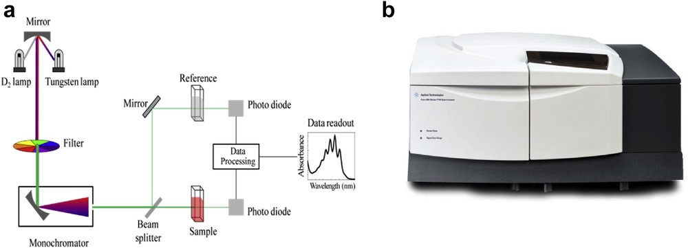
(a) Schematic for a UV–vis spectrophotometer, and (b) commercial UV–vis spectrometer from Agilent.
2.3 Calorimetric methods
Calorimetry has been a widely applied tool in the field of spin-transition materials because this technique accesses the energy relationship between the different states [34,35]. Principally, calorimetric techniques provide the thermodynamic parameters (enthalpy and entropy) associated with the spin transition, along with the transition temperature and recently with light irradiation [36].
To provide more detail about this exciting methodological area first we shall introduce the concept of specific heat [37]. Specific heat is a physical quantity that measures the change in the internal energy of a substance when the temperature changes. All phenomena or interactions that depend on temperature contribute to the heat capacity [38]. Therefore, the study of heat capacity is a means to obtain information about the energy levels (translational, vibrational, rotational, and magnetic) associated with these phenomena for comparison with models of solid-state physics.
In the case of solids, the thermal capacity is normally measured at constant pressure and is designated as Cp, from which the fundamental thermodynamic magnitudes, enthalpy (ΔH) and entropy (ΔS) associated with a given process, are obtained. These magnitudes are determined by integrating Cp with respect to temperature T and lnT, respectively:
In general, phase transitions in a molecular material have their origin in the joint action of phenomena occurring at the intramolecular level, in intermolecular interactions, and in the motion of the molecules. Therefore, specific heat is a powerful tool to study these phase transitions and to discern the mechanisms giving rise to them [39]. In the case of SCO, the change in spin state corresponds to a physical equilibrium between the two species, LS and HS. This is governed by the free enthalpy variation ΔG (Eq. 6), where the ΔH and ΔS are, respectively, the enthalpy and entropy variations in the system.
| (6) |
The enthalpy variation ΔH can be, as a first approximation, directly related to the electron contribution (ΔHel is estimated at 1000 cm−1 or 12 kJ mol−1). The entropy variation ΔS, which generally lies between 48 and 90 J K−1 mol−1, is decomposed into electronic (ΔSel) and vibrational (ΔSvib) contributions [32,40]. The electronic contribution accounts for about 30% of the total entropy, the remaining 70% being mainly related to the intramolecular vibrational contribution (Fe-ligand elongation, NFeN deformation). Intermolecular (phonon) vibrational modes are smaller by comparison. Because the coordination sphere of the LS state is more regular than that of the HS state, the transition LS → HS of a molecule is always accompanied by an increase in entropy.
The equilibrium temperature (T1/2) is defined as the point where there are as many LS molecules as HS molecules (ΔG = 0 and T1/2 = ΔH/ΔS).
- • Below T1/2, ΔH > TΔS (ΔG > 0), the enthalpy factor dominates and the LS state is the most stable.
- • Above T1/2, ΔH < TΔS (ΔG < 0), the entropy factor dominates and the HS state is the most stable.
Thus, an increase in the temperature favors the HS state and the SCO process is governed by entropy.
With the intention of measuring these values two major calorimetric techniques are mostly used: adiabatic calorimetry and differential scanning calorimetry (DSC) [41].
2.3.1 Adiabatic calorimetry
Adiabatic calorimetry (Fig. 6) is the classical Cp measurement technique. It is based on the thermodynamic definition of heat capacity at constant pressure. In practice, a heat pulse (ΔQ) is applied to the sample and the temperature increase (ΔT = Tf − Ti) is measured, yielding Cp as the quotient between these two quantities where their differentials are replaced by finite increments. In order for the heat capacity evaluation to be correct, it is necessary that there is no thermal contact between the sample and the environment, so that all of the energy supplied is used to change the state of the sample. Minimizing this thermal contact is the fundamental experimental requirement in adiabatic calorimetry, and the difficulty of achieving this makes it a complicated technique. It is, however, a precise technique (absolute precisions of 0.1–1% are achieved), although a large amount of sample is necessary (0.1–10 g).
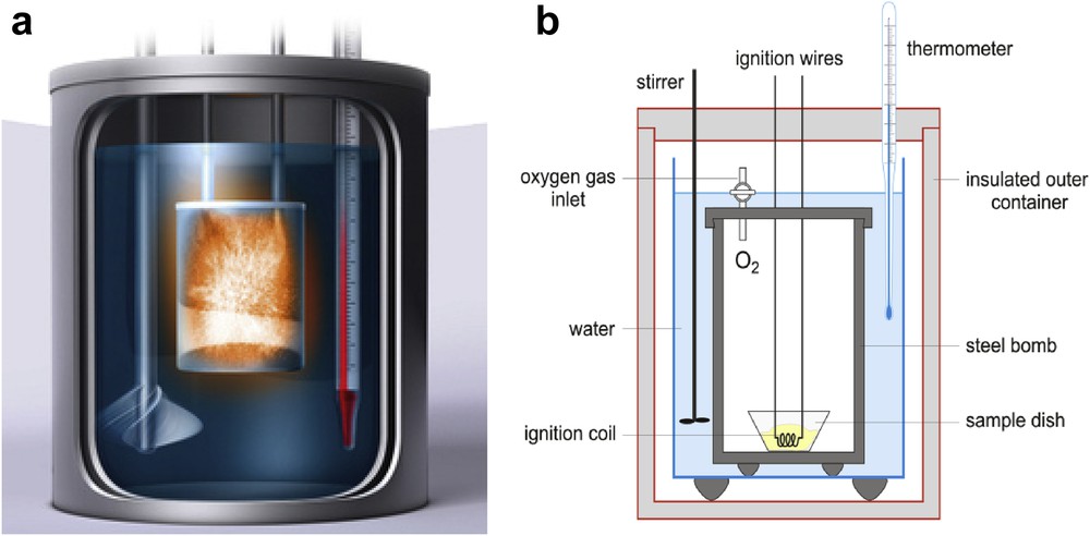
(a) General view of an adiabatic reactor, that is, illustrating the book Calorimetry: Fundamentals, Instrumentation and Applications [41]; (b) Scheme of a bomb calorimeter, in: Croatian-English Chemistry Dictionary & Glossary, 29 August 2017. KTF Split.
2.3.2 Differential scanning calorimetry
DSC consists in subjecting the same linear variation in temperature to two capsules, one a reference vacuum and the other being the sample (Fig. 7). Ideally, the difference in the power supplied to the two capsules or the temperature difference between them is proportional to the heat capacity of the sample. It is a commercially available technique and very widespread, due to its ease of use, the small amounts of sample required (on the order of 1 mg), and its speed. In contrast, its absolute accuracy is lower (1–3% at best), because measurements are not performed at a thermodynamic equilibrium, the signal is a function of the sweep rate, and measurements at temperatures below 100 K are difficult, although it has a higher application range than other techniques at temperatures above ambient.
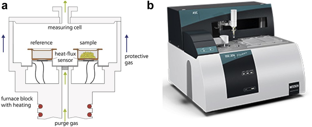
(a) Schematic view of the DSC technique. (b) DSC Phoenix Instrument (www.netzsch-thermal-analysis.com/en/products-solutions/differential-scanning-calorimetry/dsc-204-f1-phoenix)/.
3 Recent illustrative examples of SCO studies using these experimental tools
As previously mentioned, the progress made in the SCO research field has been achieved in part, thanks to the development of these methods, and also, due to the combination of different characterization techniques in the same equipment. This can be understood either from the strongly multifunctional nature of SCO or from the great effort that some research groups have made to achieve technological application with these switchable materials. This section illustrates with some examples how the state of the art in this research line has been enriched by the combination of complementary characterization methods and by increasing their sensitivity.
3.1 Increasing the sensitivity of the aforementioned techniques
Over the last decade, some research groups have successfully downsized SCO materials to the nanoscale with the aim of addressing future technological challenges [10] The successive size reductions have been accompanied by a general improvement in the sensitivity of commercially available apparatus for physical characterization. In addition, exceptional advances in data acquisition have been achieved by novel creative solutions. Probably one of the most remarkable of these examples is the design and use of a micromagnetometer prototype acting as a magnetoresistive device to measure the spin switch in very small nanosize SCO particles at room temperature [42] (Fig. 8). The change in voltage of the micromagnetometer induced by the change in the spin state of particles upon temperature variation is shown in Fig. 8.
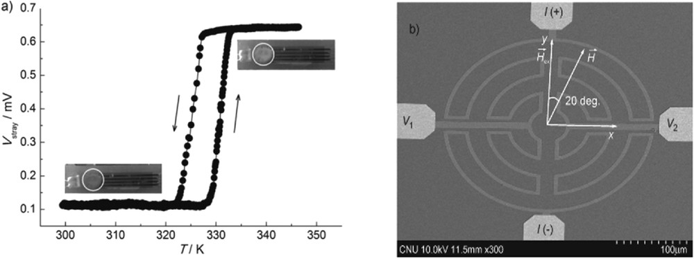
(a) The voltage change associated with the spin transition of [Fe(hptrz)3](OTs)2 nanoparticles. The diamagnetic and paramagnetic phases are characterized by lower and higher voltages, respectively [42]. (b) SEM image of a sensor junction, showing the current and voltage electrodes, applied field, and exchange-coupled field direction.
Recently, these values have been improved by using a novel version of this prototype, now reaching the highest resolution of 4 × 10⁻¹⁴ emu measured at room temperature [43]. These sensitivity values allow the sensor device to detect the SCO hysteresis loop corresponding to the lowest volume particles down to 1 × 10⁻⁴ mm3 (Fig. 9). These examples illustrate the advances in the SCO state of the art. Here, it is also important to mention that other techniques have been applied to achieve sensitivity at the molecular level. This topic will be further discussed in Chapter 7 of this special issue.
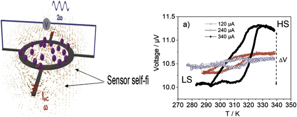
(Left) Schematic illustration of the experimental configuration showing a ring sensor with the nanoparticles (NPs) on its surface, the directions of applied current, and voltage measurement, and the self-magnetic field line represented by the small arrows. (Right) Hysteresis loop of the temperature dependence of the sensor/NP voltage: voltage change caused by the spin transition of SCO NPs for an applied current of I = 120, 240, and 340 μA [43]. The measurements were performed with a temperature sweeping rate of 2 °C min−1.
3.2 Combinations of various techniques
Probably, light irradiation has been the most widely chosen stimulus to combine with other experimental techniques to study spin transition compounds. This is because besides monitoring this phenomenon also allows obtaining a metastable state induced by light at low temperatures, the light-induced excited spin-state trapping (LIESST) effect [44,45] (which will be discussed in more detail in Chapter 3). Hence, it is worth mentioning the effort made by some research group on coupling the light to an AC calorimeter [36] and more recently, coupling it to DSC [46]. Both hybrid techniques have reported more than satisfactory results (Fig. 10).
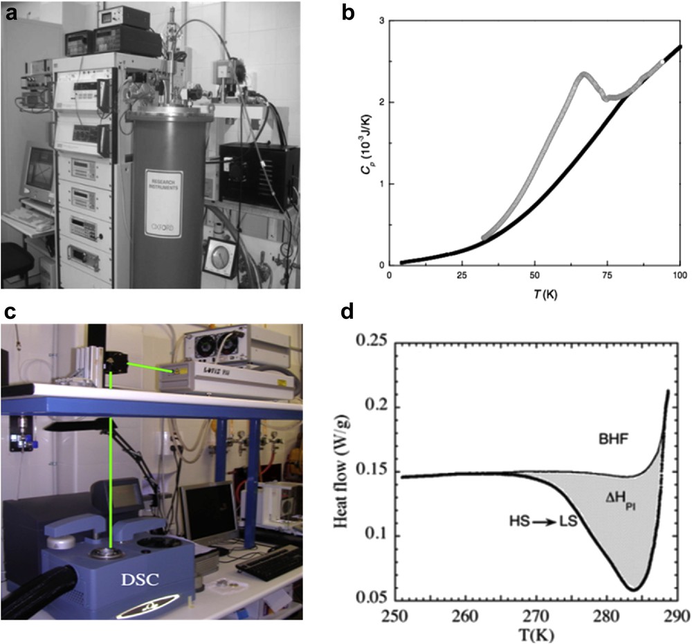
(a) Photocalorimetric AC setup. This installation permits irradiating the sample at low temperature with a Xe lamp through an optical fiber, with an estimated power on the sample of around 4 mW/cm2. (b) Heat capacity data of a pellet sample of [Fe(PM-BiA)2(NCS)2] (phase I) for the heating mode in the 5–100 K region by AC calorimetry, before irradiation (filled squares) and after 1.5 h of irradiation with 750 nm < k < 850 nm (open circles) [36]. (c) A differential scanning calorimeter model Q1000 from TA Instruments equipped with a liquid nitrogen cooling system to reach low temperature has been used. Irradiation of the sample was performed with the oven open, using commercial photocalorimetric accessories that allow illuminating the sample inside the oven when it is under the helium gas atmosphere. In (d) the process followed (see text) to deduce the enthalpy content of the photoinduced anomaly, ΔHPI, needed to estimate the HS fraction induced by the irradiation. The thick line is the calorimetric anomaly corresponding to the conversion of the photoinduced HS species to LS state, and the thin line is the background heat flow [46].
The Magnetic Property Measurement System (MPMS) from Quantum Design (USA) is one of the most popular commercially available magnetometers using SQUID technology, and it is without hesitation the most widely used characterization technique in the molecular magnetism field. The MPMS permits simultaneous measurements of the magnetic response when applying external perturbations including pressure, light irradiation, changing the chemical configuration of the materials through solvent loss, and, of course, varying the temperature. Let us look briefly at each of them.
3.2.1 SQUID coupled with a laser source
Because a handmade optical fiber was coupled with an SQUID to measure the irradiation effect on the spin transition compounds, a large number of articles have been published on the subject using a combination of these techniques [47]. Certainly, this tool has been so beneficial that now Quantum Design markets the optical fiber accessory (Fig. 11).
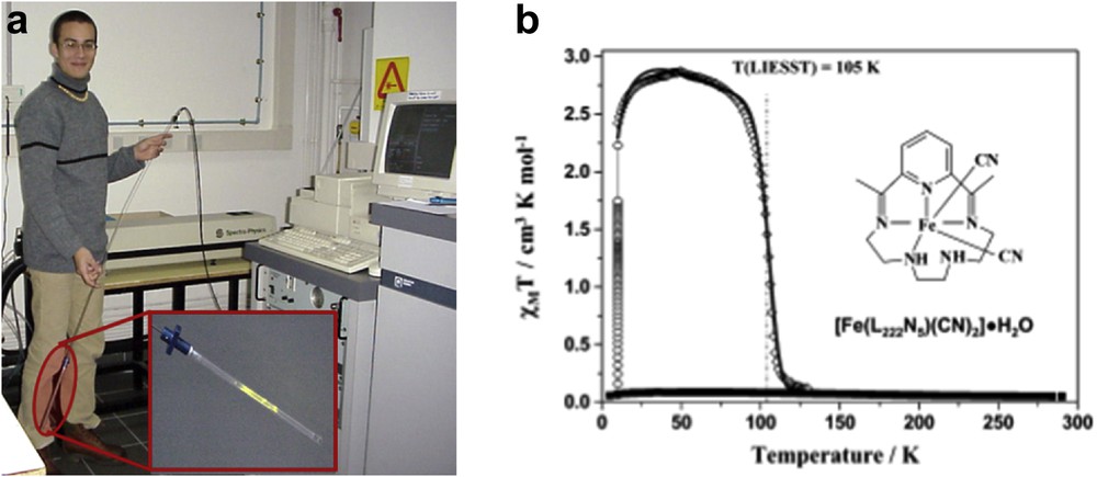
(a) MPMS SQUID coupled with a laser with filters. (b) Magnetic and photomagnetic properties recorded of a polycrystalline sample of 0.3 mg of [Fe(L222N5)(CN)2]·H2O. (■) The data were recorded in the cooling and warming mode without irradiation; (○) data recorded with irradiation at 10 K; (◊) T(LIESST) measurement, data recorded in the warming mode at a rate of 0.3 K/min with the laser turned off after irradiation for 1 h [50].
In the SCO research, this type of measurement has been associated with the measurement of the LIESST effect given a new temperature terminology called TLIESST [48,49] (see Chapter 3.2). The LIESST effect has been measured inside an SQUID for multiple SCO compounds, that is, for molecular 0D SCO [17,50] compounds as well as for 1D [51–53], 2D [54–56], and 3D [57–59] coordination polymers.
3.2.2 SQUID coupled with a pressure cell
As is known, pressure as external perturbation changes the behavior of these SCO switchable materials promoting the passage of the HS in LS electronic state (see Chapter 3.1 of this special issue). This change in the SCO properties makes these compounds of great interest for monitoring the magnetic moment change at different pressure values. Despite the major constraint of the instrument, that is, the diameter of the inner bore of the MPMS is only 9 mm, there have been several pressure cells of the piston–cylinder type built for MPMS (see quantum design Web site http://www.qdusa.com). As a result pressure can also be added as a variable for sensitive magnetization measurements (Fig. 12). Some examples using these cell pressures into the SQUID have been already compiled into a review [8,60,61] (see also Chapter 3.3). However, further progress has been carried out since their publication. In addition, thanks to this previously acquired knowledge, some compounds have been envisaged as pressure sensors for innovative applications [62].
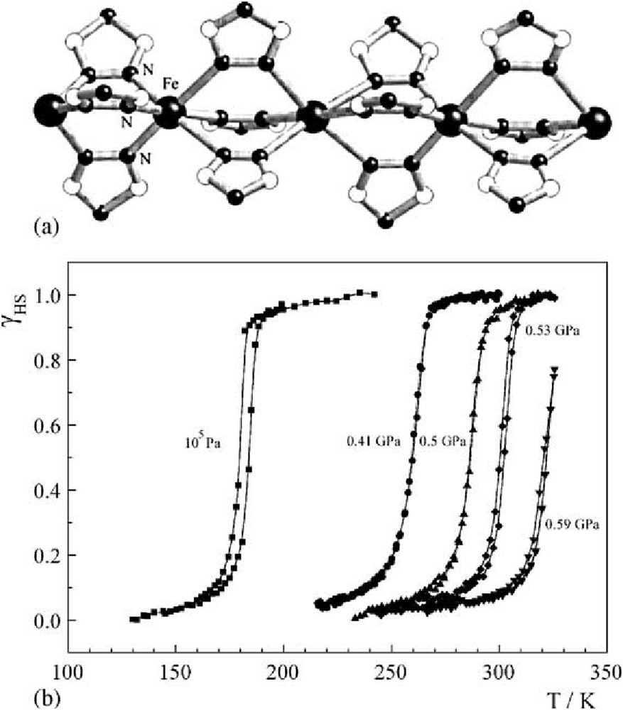
The proposed structure of the polymeric [Fe(4R-1,2,4-triazole)3]2+ SCO cation (a) and plot of γHS versus T at different pressures for [Fe(hyptrz)3](4-chlorophenylsulfonate)2·H2O (b). Reproduced with permission from Ref. [61].
3.2.3 Solvent loss effects inside an SQUID magnetometer
Modification of the chemical composition of an SCO compound may have dramatic consequences for its SCO behavior (Fig. 13). As an example, it has been reported that exchanging one water molecule inside a molecular coordination complex the SCO properties changed dramatically from a system that has no SCO behavior to the largest hysteresis loop reported for a molecular-based compound [63]. Consequently, it is of crucial relevance to monitor the magnetic variation upon changing the chemical composition of the sample. However, as far is known, a gas cell has not been coupled yet with an SQUID magnetometer. Nevertheless, it is possible to study the loss of small solvent molecules inside an SQUID just by heating the sample above room temperature and purging inside the magnetometer in a controlled manner. This measuring strategy is now commonplace and in the recent literature, some remarkable examples have been reported for both nonporous [64–66] and porous SCO materials [23,59,67–70].
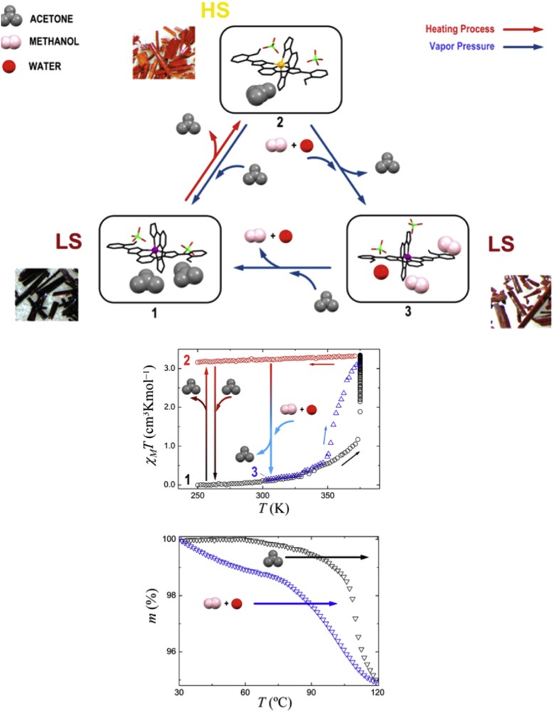
(Top) Representation of the molecular structure of 1–3 emphasizing the full conversion cycle undergone by these three species through subsequent absorption, desorption, or exchange of small molecules. Among the represented processes are the three-way proven crystal-to-crystal transformations. Pictures of the corresponding single crystals are also shown (Bottom). Plots of χMT versus T for 1 upon warming and concomitant desorption of acetone (black circles), for resulting compound 2 upon cooling (red circles), and for 3 (blue triangles, formed from 2, after substitution of acetone by MeOH + H2O) upon warming from room temperature and concomitant depletion of MeOH + H2O. The crystal-to-crystal transformations described in the text (1 → 2, 2 → 1, and 2 → 3) are shown with vertical arrows positioned, for clarity, at arbitrary temperatures. (Bottom) TGA graphs for the desorption of acetone (from 1, black symbols) and MeOH + H2O (from 2, blue symbols), emphasizing the difference in temperatures for these two processes, consistent with the observations from magnetic measurements [64].
4 Perspectives in the SCO research field due to the development of these macroscopic methods
SCO compounds are a class of functional materials containing a transition metal ion, able to reversibly switch their spin state upon external stimuli such as variations in temperature and/or pressure, magnetic field, inclusion of small molecules, and by light irradiation among others. The reversible switch between the HS and LS states make these SCO compounds ideal candidates for technological applications as molecular-based memories, nanothermometers, or sensors. Despite these extremely interesting features of SCO materials, their technological application has not been effective yet, because crucial obstacles need to be overcome before successful industrial developments can be achieved. These obstacles mainly derive from the necessity to detect the molecular phenomena unequivocally in very small objects, at the nanolevel and even further at the atomic level. To achieve this challenge the development of novel and improving the already known experimental procedures is of critical task. Along this work, we have tried to illustrate how important three techniques have been important in the SCO field and, of course, to illustrate how critical is to carry out a multidisciplinary research.
Acknowledgments
J.S.C. is grateful to Dr. Enrique Burzuri for helpful discussions. I also wish to express my sincere thanks to the Spanish MINECO for financial support through National Research Project (CTQ2016-80635-P) and the Ramon y Cajal Research program (RYC-2014-16866) for funding support. IMDEA Nanociencia acknowledges support from the “Severo Ochoa” Programme for Centres of Excellence in R&D (MINECO, Grant SEV-2016-0686)