


 CC-BY 4.0
1. Introduction
Biomass when burned properly could be considered as a renewable and an environmentally friendly source of energy. Indeed, it can be used for the generation or the cogeneration of heat and/or electricity [1]. Biomass combustion is relatively complex to model due to the presence of reaction at different phases involving charcoal, tars and volatile mixtures of organic compounds. Moreover, the presence of large amounts of ash and minerals are a source of corrosion and slagging inside the combustion chamber. However, fixed bed reactors powered by solid fuels offer high automation and low costs. The Modelling and experimentation on the complex phenomena inside these reactors and the solid biomass conversion process must address the coupling of different processes, including heat and mass transfer, gas flow, moisture evaporation, pyrolysis and the combustion and the gasification processes. Yet, Computational Fluid Dynamics (CFD) of biomass combustion can provide important insight, and often complementary information to experiments, to these complex processes [2, 3, 4].
Details on the Modelling of biomass combustion as well as on the solid phase and on the gas phase reactions are reported in the literature [5, 6, 7, 8, 9, 10, 11, 12, 13, 14]. Typically, a configuration consisting of two coupled zones (the bed and the free-board) is considered [15, 16, 17] in which the two zones are separated by an interface allowing mass and energy exchanges [2, 6, 17, 18, 19, 20]. Two general types of models are incorporated that are associated with the homogeneous and heterogeneous phases of the process [5, 18, 21]. Based on the solid phase combustion in the heterogeneous models, one may use continuous models (macro-scale models), which treat the solid phase as a porous medium [6, 10, 18, 22] and discrete element models (DEM) (micro-scale models), which describe particles in a moving grate [18, 23, 24]. Currently, most studies have focused primarily on the solid phase combustion in fixed beds, but, the simultaneous Modelling of both the solid and the gas phases is still needing more attention [5, 6, 11, 13, 22, 25, 26, 27].
Gollaza et al. studied a transient 3D CFD model for the combustion of densified wood [6]. The computational domain was divided into two zones: a fixed bed described as a porous medium and the freeboard. They simulated both the gas and the solid temperature profiles at different positions inside the reactor. Their results reproduced many of the key features of the experiments. Mehrabian et al. [5] developed a transient 3D CFD model for biomass combustion in similarly coupled zones (fixed bed and freeboard). The authors also measured the gas concentrations of CO, CO2, CH4, H2O, H2 and O2 and the temperature at various heights in the reactor for both the bed and the freeboard. Moreover, they evaluated the reaction front velocity. Their predicted results were also in a good agreement with experiments. Sun et al. [28] carried out a 2D unsteady CFD using municipal solid waste in a fixed bed reactor. They showed that their predictions of the gaseous species emissions CO, CO2, O2 and CH4 and the temperature profiles at different heights as a function of time for different moisture content were also in agreement with experimental data. These above studies underscore the importance of coupled 2-zone models for fixed bed reactors.
The objective of this study is to investigate numerically the combustion of pellets prepared from oleic by-products, and more precisely, Olive Pits (OPi) in a 40 kW counter-current fixed bed reactor. Indeed, Olive solid wastes (Olive Pomace and Olive Pits) when dried and free of residual oil, could be blended with woody biomass and densified as pellets, briquettes or logs in order to be used as fuels for feeding boilers, stoves and furnaces in many countries such as Spain and Italy. This energy policy is justified by the renewable character of the biomass and by its high heating value reaching 19 MJ/kg. Hence, it is highly important by the present study to simulate the combustion of OPi in a fixed bed reactor in order to give guidance later on the reactor design and geometry, the manner of feeding it by the primary and the secondary air, and on the level of gaseous emissions that should be reduced.
The simulations based on a cylindrical reactor are implemented using a transient 2D configuration using the COMSOL Multiphysics software. Consistently with earlier studies, the computational domain was divided into two zones: the bed and the freeboard zones. Due to the strong coupling of the mass and heat transfer between the two zones, equations describing the various sub-models were solved simultaneously to represent moisture evaporation, VOC devolatilization, pyrolysis, gasification, gas phase combustion and residual char combustion. The homogenous gas phase reactions are modelled for a fuel mixture of CO, CO2, O2, CH4, H2 and H2O in the freeboard zone. A weak turbulence 𝜅−𝜀 model is used for turbulence closure. From the simulations, we report the temperature profiles at different heights inside the reactor in the two regions and the gaseous emissions and the mass loss as a function of elapsed time. The CFD were validated using experimental data from a prior experiment [29] as well as additional data reported in the literature [5, 11, 22, 28, 30, 31, 32].
2. Model description and hypothesis
2.1. Computational configuration and modelling assumptions
The 2D axisymmetric model used is a cylindrical geometry with 400 mm height (H) and 115 mm diameter (d) is shown in Figure 1. The cylinder is divided into two zones: the fixed bed denoted (D1) and the freeboard (D2).
The 2D geometry model.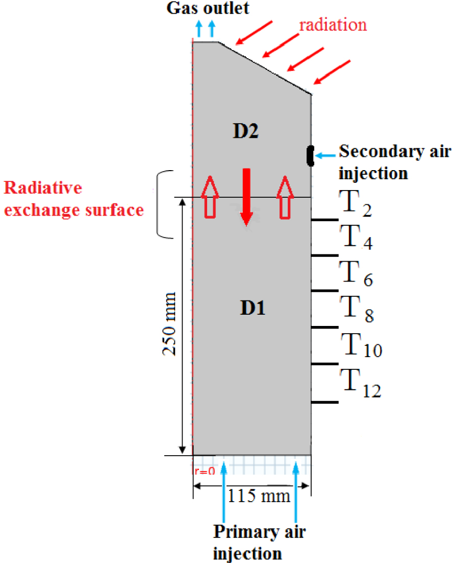
The model used to simulate the entire combustion process is based on the following assumptions and conditions:
- The computational domain is divided into two fully coupled zones: the fixed bed and the freeboard.
- The fixed bed is bounded by adiabatic walls and treated as a porous medium.
- In the counter-current configuration, the ignition starts from the top towards the bottom of the bed during which the combustion evolves layer by layer.
- The solid phase and the gas phase are modelled with their own energy equation while allowing for mass and energy exchange between the two zones via a permeable interface.
- The biomass particles are modelled as perfectly spherical and randomly packed.
- The evaporation process occurred at a specific temperature and is assumed thermally controlled.
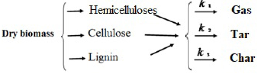
- The pyrolysis phase of the Olive Pits pellets (OPi) is modelled by a three-step reaction mechanism yielding biogas, tars and Volatile Organic Compounds (VOC).
- The solid fraction and the particles’ sizes vary during the residual char combustion and gasification.
- VOC produced during pyrolysis and gasification is mainly CO, CO2, H2, CH4 and H2Ovap. The combustion of the residual char (in the bed zone), CO, H2 and CH4 in the freeboard zone governs the entire process.
- The residual char obtained by pyrolysis is gasified by CO2 and H2O and oxidized by air. A flame front starts at the top bed and propagates to the bottom with a characteristic speed.
- No assumptions are used concerning the heat transfer and the three modes; conduction, convection and radiation are considered. The radiative transfer is modelled using an effective thermal conductivity.
- The gas emissions and the heat leaving the packed bed (D1) are considered as the inlet conditions for the freeboard zone (D2).
- The bed, which is electrically heated in the experiment, is assumed to be heated by incident radiative transfer from the walls with a prescribed constant wall temperature, Twall, equals to 1173.15 K.
- The incoming radiation flux from the freeboard region is modelled as an incident radiative heat to the fixed bed.
The reactor is fed by two air inlets: the primary air with a flow rate of 10 Nm3/h is injected under the bed bottom and passes through the fixed particles. Whereas the secondary air used to enhance the gas phase combustion is introduced at the side of the freeboard zone with a flow rate of 25 Nm3/h as illustrated in Figure 1. Both air injections occur at an ambient temperature of 298.15 K. In the actual experimental study [29], the fixed bed was equipped with thirteen type K-thermocouples, which are spaced at 20 mm increment along the reactor, but, only six type K-thermocouples (Figure 1) are considered during the present numerical study in order to reduce the simulation time.
2.2. Modelling of rate processes
The overall combustion process can be divided into four different sub-processes: drying, pyrolysis and combustion of VOC, and combustion and gasification of the residual char. In this study, the drying process is modelled as a heterogeneous reaction at the solid temperature [32, 33, 34]. This process is represented by a first-order kinetic reaction based on the Arrhenius law:
| (1) |
| (2) |
| (3) |
Rate constant’s parameters
| Olive pits pellets | Pre-exponential factor A (1/s) | Activation energy E (kJ/mol) |
|---|---|---|
| Drying | 1.06 × 10³ | 88.5 |
| Pyrolysis | ||
| Cellulose | 2 × 10¹² | 185 |
| Hemicellulose | 3.5 × 10¹¹ | 105 |
| Lignin | 108 | 192 |
| Tar | 1.5 × 10⁵ | 192 |
| Residual char combustion | 9 × 10⁸ | 2.25 × 10⁵ (k1) |
| 7 × 10⁹ | 1.3 × 10³ (k2) | |
| Residual char gasification | 1.6 × 10⁶ | 2.2 × 10⁴ (k3) |
| 3.5 × 10⁷ | 225 × 104 (k4) | |
| Combustion of pyrolysis gases | 107 | 1.89 × 10⁵ (k5) |
| 1.674 × 10⁵ | 1.25 × 10³ (k6) | |
| 1.95 × 10⁷ | 1.67 × 10⁵ (k7) | |
Pyrolysis is a complex process, which involves a number of coupled chemical reactions [10, 35, 36, 37, 38]. Here, the lignocellulosic samples containing mainly hemicelluloses, cellulose and lignin produce, via pyrolysis, three products; biogas, tars and biochar. The rate contents of these products depend on the type of samples and especially on the type of pyrolysis (slow, fast or flash). The total devolatilization rate [34] is modelled as follows:
| (4) |
The reaction of the combustion and gasification of the residual char is considered as a heterogeneous and exothermic reaction [39, 40]. The oxidation of the residual char with the O2 of injected primary air is described by the following 2-step reactions:
| (5) |
| (6) |
| (7) |
| (8) |
| (9) |
| (10) |
| (11) |
| (12) |
The combustion of gaseous emissions is modelled using the following reactions:
| (13) |
| (14) |
| (15) |
2.3. Governing equations in the fixed bed and the freeboard
Solid and gas phase equations are solved as a transient two-dimensional formulation in cylindrical coordinates. Various conservation equations describing the fuel conversion of mass, momentum and energy were solved in two coupled zones as reported in literature for similar studies [2, 3, 4, 10, 11, 12, 13]. The gases emitted from the bed, CO, CO2, H2 and CH4, and their composition are prescribed as inlet conditions for the freeboard zone. These gases are likely to react with oxygen in the secondary air. In order to lighten the text to the readers, all equations with meanings of all variables and parameters are provided in Appendices A and B.
2.4. Fuel properties
The size of the olive solid by-products pellets as olive pits used in our numerical simulation ranged from approximately 2.5 to 3.5 cm and with an equivalent diameter up to 6 mm. Ultimate analysis as %C, %H, and %O and proximate analysis as Volatile Matter (%VM), %Ash and Fixed Carbone (%C) and energy contents as the bulk density of the olive solid by-products pellets are assumed to be the same as the values published in [29]. On the other hand, the ash content evolution is not taken into account.
2.5. Mesh and numerical resolution
The finite element method was used to discretize the unsteady governing equations. To establish grid convergence, we considered 5 mesh resolutions, which are summarized in Table 3.
Calculations show that the meshes named coarse or normal did not yield grid convergence. However, finer or extra-fine meshes required extensive computational times four to five weeks on a mini-workstation. The “fine” mesh resolution provides a reasonable compromise where grid convergence is established while a reasonable computational time of approximately 24 h is achieved. The corresponding mesh size is approximately 1.5 mm, whereas the calculation time was automatically defined by the solver.
Finally, a moving mesh was adopted in order to refine our calculations at the interface between the two computational zones as shown on Figure 2.
Mesh grid structure.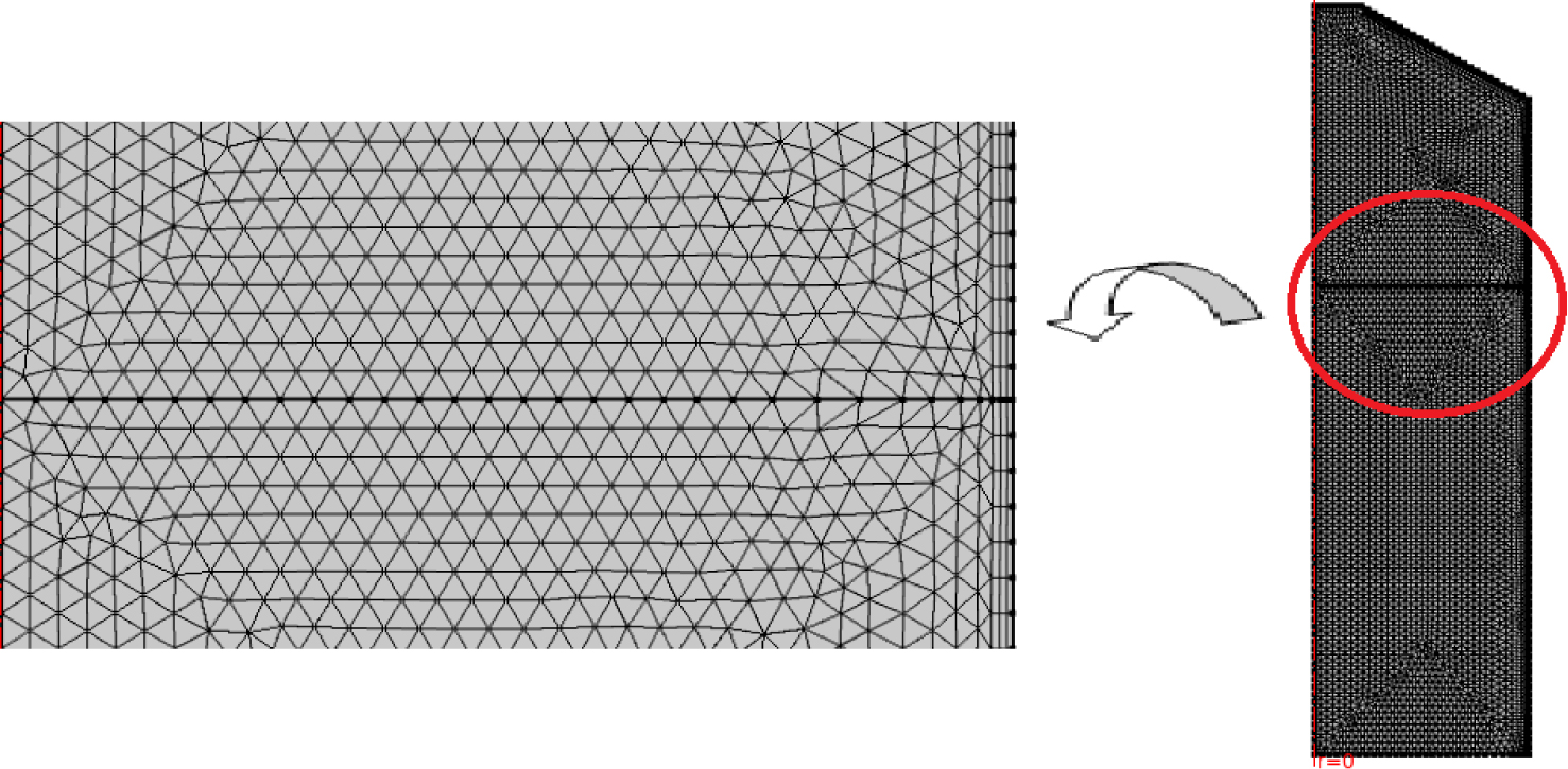
3. Results and discussion
3.1. Mass loss
The accurate prediction of the temporal evolution of the mass loss of the olive pit pellets is an important test of the overall performance of the computational study. This mass loss is prescribed by the following equation:
| (16) |
Figure 3 compares the temporal evolutions of the modelled (dashed) and measured (solid) mass loss [29]. The comparison shows a good agreement between measurements and computations. The mass loss could be divided into three phases (I), (II) and (III) on Figure 3: the first phase (I) corresponds to moisture evaporation, the second phase (II) corresponds to the devolatilization and combustion of gases, and. the final phase (III) corresponds to the residual char combustion. Similar results were reported in literature for both numerical simulations [14, 45] and experimental measurements [46, 47, 48].
Mass loss history. Experiment (solid), Simulation (dashed).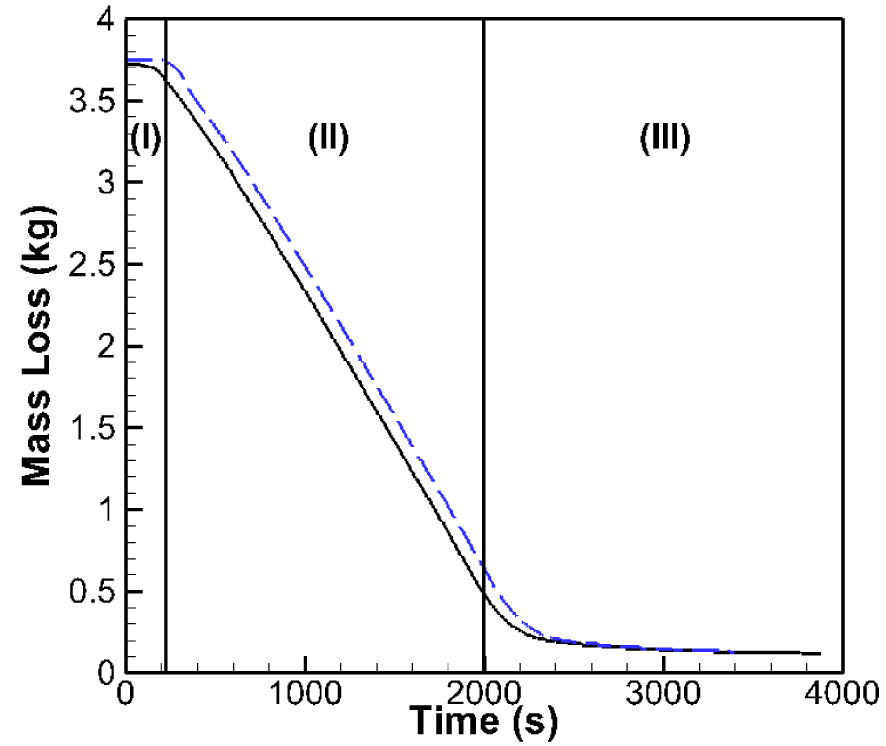
Different mesh resolutions considered with their boundary and domain elements
| Meshes | Domain elements | Boundary elements |
|---|---|---|
| Coarse | 2,129 | 154 |
| Normal | 4,525 | 224 |
| Fine | 7,305 | 285 |
| Finer | 11,176 | 354 |
| Extra-fine | 49,944 | 748 |
3.2. Temperature and gas velocity evolutions inside the reactor
The temporal evolution of the temperature distribution inside the reactor is shown in Figure 4. The figure also serves to highlight the propagation of the combustion processes both in the freeboard zone and in the fixed bed. As shown, ignition started from the top at t = 0 s, and then the flame propagates rapidly in the gas phase. This process continues into the solid phase, yet at a slower rate, until the bottom of the bed is reached [31].
The temperature distribution inside the reactor at different instants.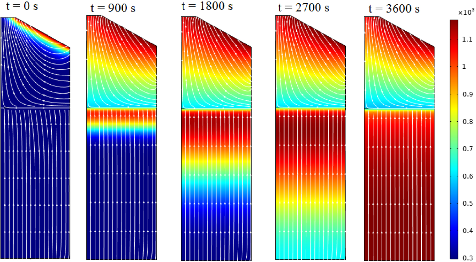
However, the gas velocity profile as a function of the radial distance of the reactor, as illustrated in Figure 5, reveals that the gas flows in the opposite direction to the ignition front propagation, hence, the counter-current nature of the bed [49]. The decrease of the temperature near the interface between the gas and solid phases can be attributed to convective cooling associated with secondary air [26, 50]. For a height up to approximately 0.3 m, the gas velocity profile remains flat (≈0.075 m⋅s−1). However, as the mixture of gases and secondary air reach the activation temperature, the combustion in the gas phase is started and the gas velocity increases rapidly reaching about 5 m/s. This is a typical value for gas phase combustion [26].
Gas velocity profile.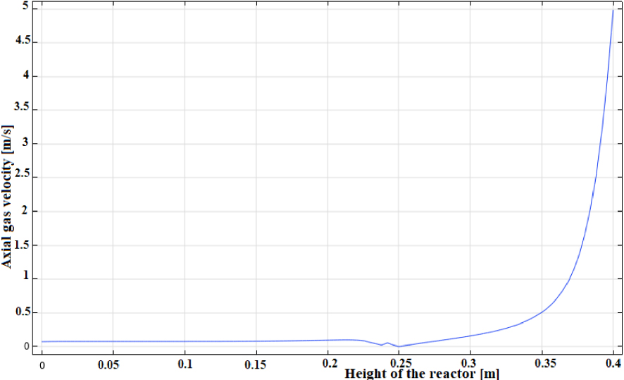
To better understand the combustion process in the fixed bed, we attempt to look closely at the solid phase combustion. Figure 6 compares the computed and measured temperature profiles of the olive pit pellets at different heights along the reactor centreline corresponding to 5, 45, 85 and 165 mm, which also correspond to 4 different placements of the thermocouples in the experiment [29, 51]. The simulation was undertaken under the same experimental conditions with a primary air flowrate of 10 Nm3/h injected at ambient conditions (105 Pa, 298.15 K). The secondary air flowrate was 25 Nm3/h under the same standard conditions of temperature and pressure. The figure shows a reasonable agreement between computation and experiment, exhibiting both similar temporal trends and magnitudes.
Comparison of temperature profiles obtained numerically and experimentally. Experiment (solid), Simulation (dashed).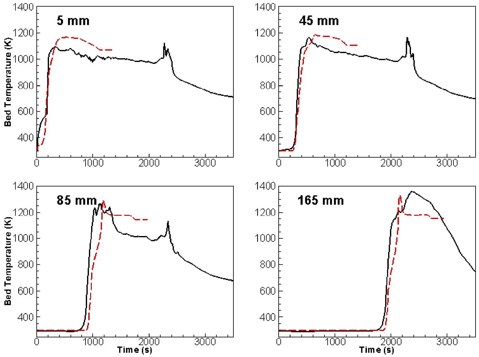
The discrepancy between experimental and simulated temperature (overestimation of its maximum) can be attributed to two possible sources. First, radiative absorption is not taken into account in our computations. Species like CO2, CO and water vapour are characterized by reasonably high absorption coefficients. Second, the presence of ash subject to melting and agglomeration at high temperatures may inhibit the air circulation through the porous medium. Nevertheless, these results show again that the self-sustained progression of the combustion front evolves from the upper to the lower layers of the bed. In addition, the appearance of an odd little peak at a given time for every fixed bed depth corresponds to the condition of maximum efficiency of reactivity because of maximum yields of CO, H2 and Corg as it is shown on Figure 8. Consequently, there is a maximum heat release by reactions manifesting with a maximum temperature.
Figure 7 compares computed temporal evolutions of temperature of the solid and gas phases inside the fixed bed (zone D1) at the 5 different thermocouple positions corresponding to 2, 45, 85, 165 and 205 mm. The result shows that both solid and gases phases are in thermal equilibrium inside the porous medium. Hence, it is possible to consider a single energy conservation equation and to exclude the convective term between the gas phase and the solid phase. Such an assumption can greatly simplify the model formulation and improve the efficiency of the computations.
Simulated temperatures of the solid and gas inside the fixed bed (D1 zone). Solid temperature (solid), gas temperature (dashed).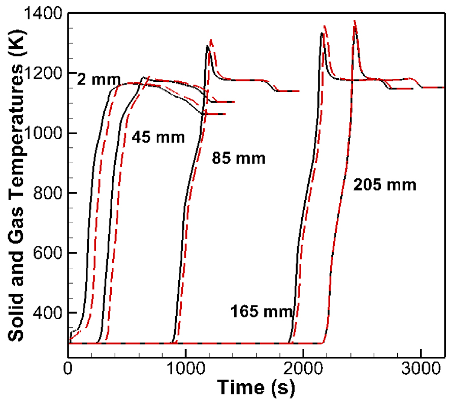
3.3. Gaseous emissions in the freeboard zone
Figure 8 compares the temporal evolutions of the computed and measured gaseous emissions for O2, CO, CO2, H2, CH4, H2Og, and Corg whenever such comparisons are available. We observe the presence of discrepancies between simulated and experimental profiles: There is temporal delay between curves and simulated profiles do not exhibit the fluctuations observed in the experimental results. We believe that the discrepancy may be attributed to ash accumulation, which prevents the inlet air circulation. Moreover, the physical presence of thermocouples could affect measurements, but above all, the kinetics of reactivity should be improved.
Gaseous emissions in the freeboard zone: comparison between simulated and experimental results. Experiment: Solid, Simulation: Dashed.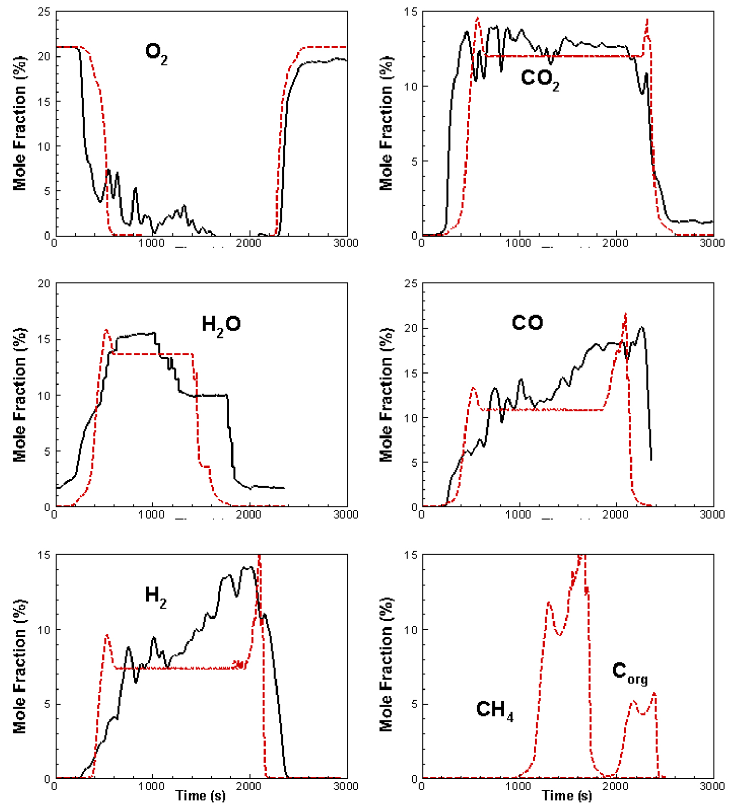
The increase of water vapour concentration can be attributed to the fuel evaporation and to the combustion of H2 and CH4 as shown in (15) and (18). Moreover, the sudden decrease of O2 concentration marks the onset of the combustion process. This process is accompanied by an increase in CO2 and CO concentrations. One observes that the concentration of CO2 increases rapidly and remains at a roughly constant level of about 15% (against around 14% for the experiment measurements). In contrast, the increase of concentration of CO and H2 could be explained by the gasification of the residual char in the presence of gasifiers CO2 and water vapour, not to mention the contributions of CH4 reactions described by (9), (10) and (15). Moreover, the behaviour of methane gas is similar to what was reported in some numerical simulation studies in literature [4, 44, 52]. A decrease in H2O, H2, CO and CO2 was noted at the end of the combustion process (the fuel is completely consumed), while the O2 mole fraction is again 21%.
Regardless, the slight difference between the simulation and the experiment in Figure 8 can be due to the sub models associated with the flow, turbulence and chemistry as well as the choice of the axisymmetric geometry. Also, during the experiment measurements certain systematic and non-systematic errors may be at the source of some fluctuations.
4. Characteristic parameters
Some characteristic parameters, which describe the combustion behaviour including the reaction front velocity, the mass conversion rate and the ignition rate are obtained from the measurements can be modelled. The comparisons of the temporal evolution of these parameters are shown in Figures 9a and b as a function of time. The comparison between these measurements and calculated parameters shows a relatively good agreement. However, these dependencies characteristics can provide a basis to transfer the fixed bed reactor to the situation of a grate incinerator.
(a) A comparison between the measurement and the calculated of the reaction front velocity. (b) A comparison between the measurement and the calculated of the mass conversion rate and the ignition rate.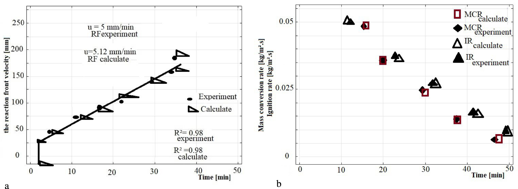
5. Main variables evolution in the model
Finally, we present profiles of the mass densities of the solid fraction (top left), the char density (top right), the moisture density (bottom left) and the dry olive pits pellets density (bottom right). These computed profiles are compared to those of the experiment in Figure 10. These modelled results correspond to the CFD simulations for the fixed bed reactor (zone D1) at time t = 3900 s and a primary airflow equal to 310 kg⋅h−1⋅m−2. The figure shows that a large zone of char density remains constant at the vicinity of 170 kg⋅m−3. In this large zone, the primary airflow injection may not have been sufficient for a rapid consumption of the generated char. Consequently, this may have delayed the homogenous reaction of the char. This observation was also reported in the literature for the same conditions of airflow (0.05 kg⋅s−1⋅m−2) [49].
Evaluation of solid fraction and densities of char, moisture, and dry olive pits pellets at 3900 s.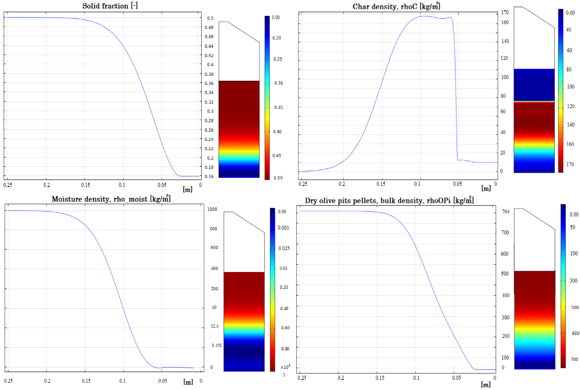
6. Conclusion
A transient 2D axisymmetric CFD simulation was carried out to simulate the multiphase combustion of lignocellulosic solid biofuels (olive pits pellets) in a counter-current fixed bed reactor. The simulations were implemented using COMSOL Multiphysics 5.5. The reactor is divided into two zones: D1 and D2 representing the fixed bed and the freeboard. Reduced kinetic schemes were used in the solid and the gas phases. Moreover, an Euler/Euler approach was used to model the porous fixed bed. The turbulent flow was described by the k −𝜀 model. Results show that the present formulation adequately reproduces experimental observations related to over-the-bed gas concentrations, temperatures and mass loss. Calculated characteristic parameters like reaction front velocity, mass conversion rate and ignition rate are reproduced in close agreement with the experiment. However, the models developed for the pilot scale fixed bed reactor can be extended to an industrial-scale plant for example using an incinerator grate.
Nomenclature
| u | Velocity | m⋅s−1 |
| A | Pre-exponential factor | s−1 |
| D | Diffusion coefficient | m2⋅s−1 |
| Y | Mass fraction | – |
| Si | Source term | kg⋅m−3⋅s−1 |
| p | Pressure | Pa |
| g | Gravitational acceleration constant | m⋅s−2 |
| Cp | Specific heat | J⋅kg−1⋅K−1 |
| S | Surface | m−2 |
| h | Convective heat transfer coefficient | W⋅m−2⋅K−1 |
| 𝛥HR | Enthalpy of reaction | J⋅kg−1 |
| Qrad | Radiative source | W⋅m−3 |
| d | Diameter | m |
| E | Activation energy | J⋅kmol−1 |
| Sk | Source term of the turbulent energy production | kg⋅m−1⋅s−3 |
| S∈ | Source term of turbulent dissipated energy | kg⋅m−1⋅s−4 |
| T | Temperature | K |
| X,x | Mole fraction | – |
| R | Ideal gas constant | J⋅mol−1⋅K−1 |
| Reaction rate | kg⋅m−3⋅s−1 | |
| t | Time | s |
| H | Reactor height | m |
| z | Axial position | m |
| r | Net production rate of the gas species | kg⋅m−3⋅s−1 |
| M | Atomic molar mass | kg⋅mol−1 |
| Nu | Nusselt number | – |
| Re | Reynolds Number | – |
| Pr | Prandtl Number | – |
| k | Turbulent kinetic energy | m2⋅s−2 |
| KR | Permeability | m2 |
| r | Radial position | m |
| Air flow | kg⋅s−1 | |
| a | Bed cross-section | m2 |
| ki | Kinetic rate constant | s−1 |
| f | Pressure loss | N⋅m−3 |
Greek symbols
| 𝜀 | Porosity | – |
| 𝜆 | Thermal conductivity | W⋅m−1⋅K−1 |
| 𝜇 | Dynamic viscosity | Pa⋅s |
| 𝜌 | Density | kg⋅m−3 |
| 𝜎 | Stefan–Boltzmann constant | W⋅m−2⋅K−4 |
| ∈ | Turbulent kinetic energy dissipation | m2⋅s−3 |
| 𝜆 | Stoichiometric air coefficient | – |
| 𝛽 | Absorption coefficient | – |
| 𝜔 | Emissivity | – |
| 𝛼 | Mass of the compound i produced per kg of pyrolyzed | – |
| 𝜎i,j | collision cross-section | Å |
| 𝛺i,j | collision integral | – |
| 𝜏i,j | Stress tensor | – |
Subscripts
| app | Apparent |
| eff | Effective |
| t | Total |
| rad | Radiation |
| pyr | Pyrolysis |
| g | Gas |
| s | Solid |
| i,j | Relating to components I and j |
| p | Particle |
| v | Vaporisation |
| a | Ash |
| c or C | Carbon |
| CFD | Computational Fluid Dynamics |
Conflicts of interest
Authors have no conflict of interest to declare.