

1 Introduction
In soils, FeIII species are very frequently trapped in solid iron oxyhydroxides. In contrast, FeII species move much more rapidly because they are easily dissolved. Therefore, the understanding of the possible chemical reactions that occur at the solid/solution interface between FeII dissolved species and the various ferric oxyhydroxides is fundamental. It is now well established that dissimilatory iron reducing bacteria (DIRB) play a major role in the biogeochemical cycle of iron, because they are responsible for the reductive dissolution of ferric oxyhydroxides FeOOH. Once FeII dissolved species are produced by the bacteria, a reaction of coprecipitation between FeII species and the FeIII species remaining into FeOOH may occur and mixed FeII–FeIII compounds form. Such coprecipitation reactions between FeII and FeIII species were studied in abiotic conditions by several authors, e.g., [2,8,9,12,15–17]. It was namely shown that FeII species react easily with lepidocrocite (or ferrihydrite) to form either green rust [8,16] or magnetite [9,12,17] and that the adsorption of hydroxylated FeII species on the surface of the ferric oxyhydroxide FeOOH was an initial step that precedes the formation of magnetite [15,17]. In FeIII rich medium, the formation of magnetite Fe3O4 was favoured, but was sometimes preceded by the precipitation of green rusts [12,15]. It is now well established that in anoxic conditions green rusts are transformed either in a mixture of magnetite and siderite {Fe3O4, FeCO3}, when carbonate anions are present [3,5], or in a mixture of magnetite and ferrous hydroxide {Fe3O4, Fe(OH)2} [14] at pH higher than 9.
By using the experimental method used in the early work of Arden [2], reactions of coprecipitation were studied systematically by performing the titration of various FeII–FeIII solutions [14]. A mass-balance diagram was shown to be a powerful tool to study the various steps of the reaction and the properties of this diagram are explained here. The formation of hydroxycarbonate green rust and Al-substituted hydroxysulphate green rust by coprecipitation was also studied recently [1,5].
2 Experimental method
The samples were prepared by the coprecipitation of FeII and FeIII species in different kinds of aqueous solutions. This simple method, which consists to add a basic solution to a mixture that contains FeII and FeIII dissolved species, is well known for the synthesis of the other members of the layered double hydroxides (LDHs) family. Due to the fact that the divalent cation FeII can easily be oxidised, the evacuation of dissolved oxygen was ensured by a continuous N2 bubbling in the aqueous solution introduced in a gas tight reactor. The initial solution was prepared by dissolving in demineralised water appropriate amounts of FeII and FeIII salts. A basic solution was progressively added to the initial mixture by using a peristaltic pump at a constant flow rate of ∼0.5 ml min−1. The duration of the experiments was ∼5 h and the pH of the solution was monitored continuously. Depending on the type of samples that was synthesised, different methods were used that are summarised in Table 1. The suspensions were filtered under an inert atmosphere and the precipitates were analysed by several techniques: X-ray diffraction (XRD) at a wavelength
Conditions of preparation of the samples synthesised by coprecipitation: hydroxysulphate green rust {GR(
Conditions de préparation des échantillons synthétisés par coprécipitation : rouille verte sulfatée {GR(
| Type of green rust |
|
|
Salts and concentration of the initial solution | Base |
| GR( |
0; 0.1; 0.14; 0.17; 0.2; 0.25, 0.33; 0.5; 0.67, 1 | 0 | FeSO4⋅7 H2O | [NaOH] = 0.8 M |
| Fe2(SO4)3⋅5 H2O | ||||
| [Fe]=4×10⁻¹ M | ||||
| GR( |
0, 0.33, 0.4, 0.5, 1 | 0 | FeSO4⋅7 H2O | [Na2CO3] = 0.57 M |
| Fe2(SO4)3⋅5 H2O | ||||
| [Fe]=6.7×10⁻² M | ||||
| GR( |
0.25 | 0 | FeCl2⋅4 H2O | [Na2CO3] = 0.57 M |
| FeCl3⋅6 H2O | ||||
| [Fe]=6.7×10⁻² M | ||||
| Al-GR( |
0.2; 0.185; 0.16; 0.1 | 0; 0.015; 0.04; 0.1 | FeSO4⋅7 H2O | [NaOH] = 0.8 M |
| Fe2(SO4)3⋅5 H2O | ||||
| Al2(SO4)3⋅5 H2O | ||||
| [Fe]+[Al]=4×10⁻¹ M |
3 Properties of the mass-balance diagram
3.1 Construction of the diagram
If one considers the mass-balance of the previously described coprecipitation experiments, the nature and the relative abundances of the iron containing compounds that form are governed by two parameters: (i) the ferric molar fraction of the initial mixed FeII–FeIII solution, i.e. the ratio
It is convenient to represent in a mass-balance diagram [14] the ratio
| (1a) |
| (1b) |
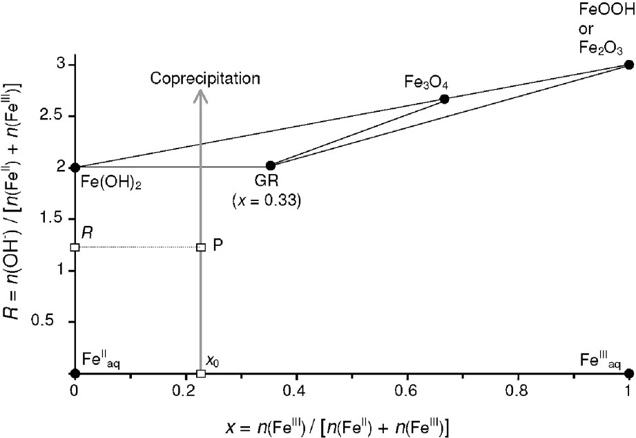
FeII–FeIII mass-balance diagram, showing the route of a coprecipitation experiment.
Diagramme bilan matière du système FeII–FeIII et représentation du chemin correspondant à une réaction de coprécipitation.
In a same manner, the position of the different solid compounds can easily be determined: ferrous hydroxide Fe(OH)2, green rust (GR) of general chemical formula
3.2 Interpreting the diagram
A coprecipitation experiment that is realised at a constant ferric molar fraction ratio
- – (a) a single compound forms if P is situated at a point
- – (b) a two-compound system forms if point P is situated on a tie-line that joins two compounds, e.g., the tie-line that joins Fe(OH)2 to GR in Fig. 1. In a general case, let us consider the formation of a mixture of two compounds α and β that correspond to the two points
(2)
where n(OH−), n(FeIII), n(OH−)[α], n(FeIII)[α], n(OH−)[β] and n(FeIII)[β] are the respective mole numbers of OH− and FeIII consumed during the formation of the whole mixture and their repartition in the α and β compounds. It can be demonstrated that Eqs. (2) and (3) are equivalent to the following equations:(3) (4) (5) It should be noted that if Mössbauer spectroscopy is performed for analysing the
- – (c) a three-compound mixture forms if point P is situated inside a triangle of three compounds, e.g., Fe(OH)2, GR and Fe3O4 in Fig. 1. Let us again consider the general case of three compounds represented by the three points
(9) The Fe molar fractions
(12) (13) (14)
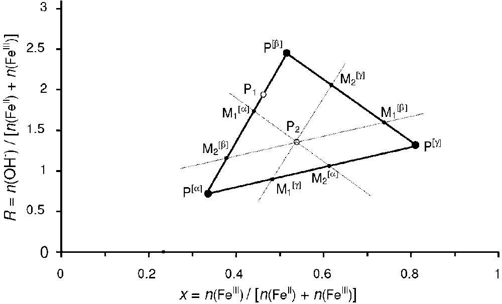
Graphical determination of the relative abundance of the compounds in the mass-balance diagram. For point P1, the two-compound system {α+β} forms and the relative quantities are given by Eqs. (7) and (8). For point P2, the three-compound system {α+β+γ} forms and the relative quantities are given by Eqs. (12), (13) and (14).
Détermination graphique des abondances relatives de chaque phase dans le diagramme bilan matière. Pour le point P1, le système biphasé {α+β} se forme et les quantités relatives de chaque phase sont données par les Éqs. (7) et (8). Pour le point P2, le système triphasé {α+β+γ} se forme et les quantités relatives de chaque phase sont données par les Éqs. (12), (13) et (14).
4 Mechanism of formation of hydroxysulphate green rust
4.1 Analyses of the pH curves
For 10 different values of the ferric molar fraction x, titration curves were presented in a previous work [14] and three typical curves are shown in Fig. 3. The curves are characterised by three plateaus separated by two equivalent points E1 and E2. For

Evolution of pH during the titration of different FeII–FeIII solutions.
Variation du pH au cours de la titration de différentes solutions mixtes FeII–FeIII.
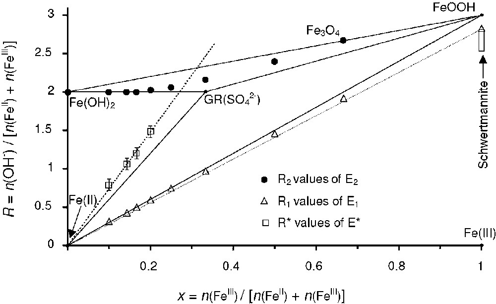
R values of equivalent points E1 and E2 and point E* presented in the mass-balance diagram.
Valeurs de R pour les différents points E1, E2 et E*, qui sont représentées dans le diagramme bilan matière.
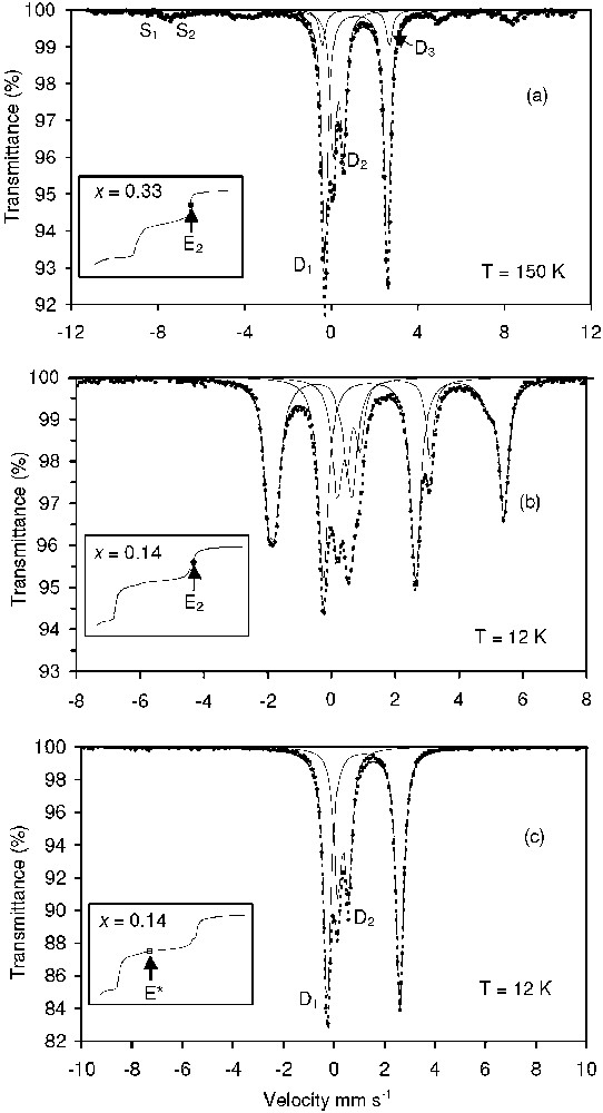
Mössbauer spectra of the solid compounds obtained at different points of the titration curves.
Spectres Mössbauer des composés solides obtenus en différents points des courbes de titration.
Hyperfine parameters of the Mössbauer spectra presented in Fig. 5
Paramètres hyperfins des spectres Mössbauer présentés sur la Fig. 5
| Spectra | Compounds | δ | Δ or |
H | FWHM | RA (%) measured | RA (%) predicteda | |
| Fig. 5a | GR( |
D1 | 1.29 | 2.87 | — | 0.32 | 53 | (D1 + D2) |
| 52 | ||||||||
| D2 | 0.48 | 0.46 | — | 0.32 | 28 | |||
| Fe(OH)2 | D3 | 1.28 | 3.09 | — | 0.32 | 8 | 24 | |
| Fe3O4 | S1 | 0.46 | 0 | 493 | 0.79 | 7 | (S1 + S2) | |
| 24 | ||||||||
| S2 | 0.86 | 0 | 468 | 0.69 | 4 | |||
| Fig. 5b | GR( |
D1 | 1.32 | 2.88 | — | 0.37 | 34 | (D1 + D2) |
| 43 | ||||||||
| D2 | 0.55 | 0.47 | — | 0.37 | 18 | |||
| Fe(OH)2b | 1.3 | −3.1 | 166 | 0.34 | 48 | 57 | ||
| Fig. 5c | GR( |
D1 | 1.32 | 2.86 | — | 0.34 | 66 | (D1 + D2) |
| D2 | 0.52 | 0.43 | — | 0.34 | 34 | 100 |
a Predicted by using the lever rules in the mass-balance diagram. Valeurs prédites en utilisant la règle des leviers dans le diagramme bilan matière.
b Simulation of this component by a mixture of quantum states according to Génin [6]. Simulation de cette composante à l'aide d'un mélange d‘état quantique d'après Génin [6].
The most interesting part of this analysis is the position of points E* observed on the pH curves when
4.2 Analyses of Fe and
The different steps of the coprecipitation experiments were analysed by measuring the concentrations of Fe, FeII and
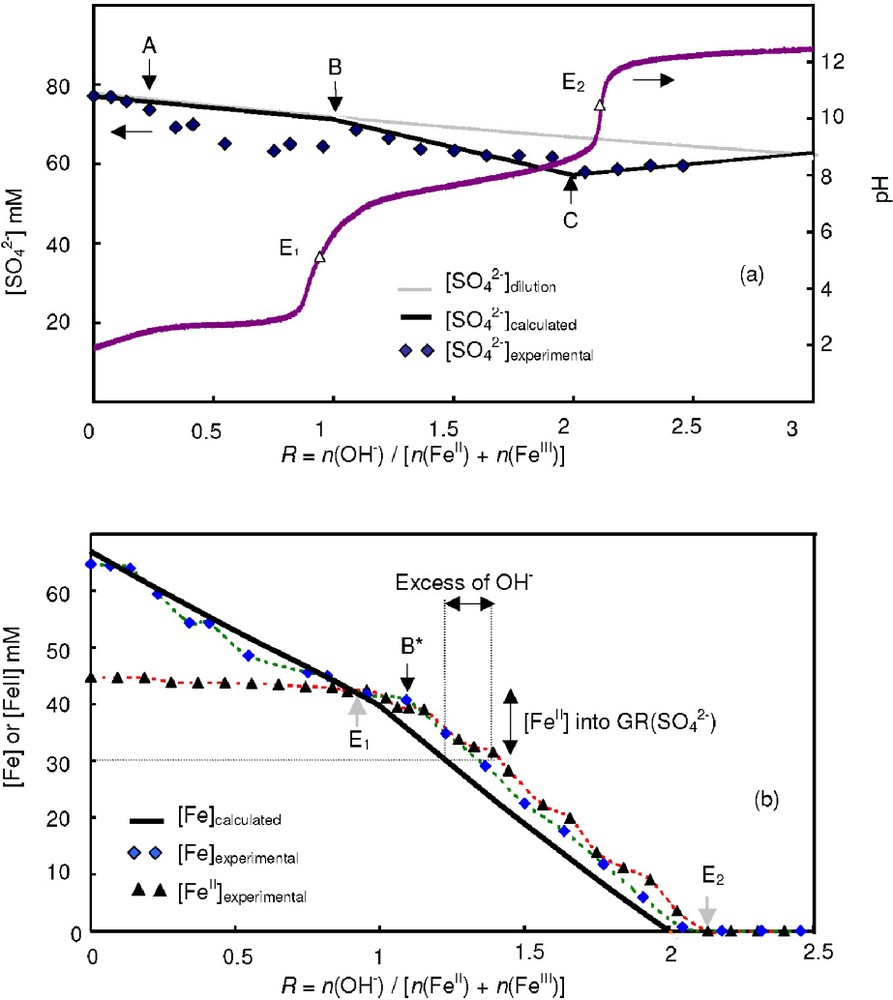
Evolution of the concentrations [
Variation des concentrations en solution [
The concentration of
The Fe concentrations measured in solution ([Fe]exp) are also situated slightly above the calculated values between points A and B confirming the formation of the ferric basic salt (Fig. 6b). By using both values
4.3 Mode of formation of GR(
Analyses of the pH titration curves performed with the mass-balance diagram, Mössbauer spectroscopy and measurements of Fe and
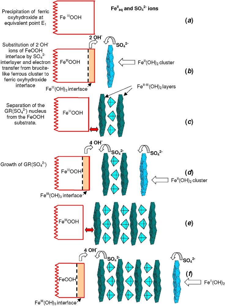
Mode of formation of hydroxysulphate green rust GR(
Mode de formation de la rouille verte sulfatée. La description des différentes étapes (a, b, c, ...) sont décrites dans le texte.
The interlayer of
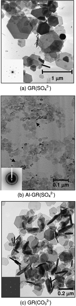
TEM images of hydroxysulphate green rust (a), Al-substituted hydroxysulphate green rust (b) and hydroxycarbonate green rust (c).
Images de microscopie électronique en transmission : (a) rouille verte sulfatée, (b) rouille verte sulfatée substituée aluminium, (c) rouille verte carbonatée.
5 Chemical composition of green rust
5.1 Hydroxysulphate green rust
FeII–FeIII solutions were precipitated by a NaOH solution at a constant ratio

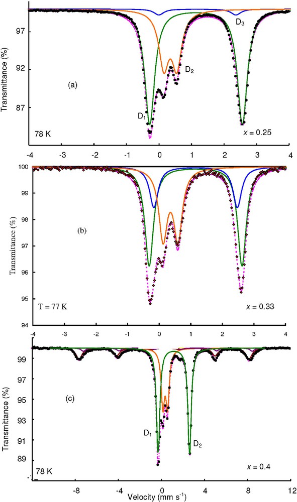
Evolution of the Mössbauer spectra as a function of the ferric molar fraction x for samples prepared in a sulphated aqueous medium at a constant hydroxylation level R=2.
Évolution des spectres Mössbauer en fonction de la fraction molaire en ions FeIII pour des échantillons préparés à un taux d'hydroxylation constant R=2.
Hyperfine parameters of the Mössbauer spectra presented in Fig. 8
Paramètres hyperfins des spectres Mössbauer présentés sur la Fig. 8
| Spectra | Compounds | δ | Δ or |
H | FWHM | RA (%) | |
| Fig. 8a | GR( |
D1 | 1.32 | 2.88 | — | 0.37 | 63.5 |
| D2 | 0.55 | 0.47 | — | 0.37 | 32 | ||
| Fe(OH)2 | 1.3 | −3.1 | 166 | 0.34 | 4.5 | ||
| Fig. 8b | GR( |
D1 | 1.35 | 2.88 | — | 0.37 | 60 |
| D2 | 0.49 | 0.5 | — | 0.37 | 35 | ||
| S | 0.69 | 0 | 474 | 0.34 | 5 | ||
| Fig. 8c | GR( |
D1 | 1.32 | 2.86 | — | 0.55 | 40 |
| D2 | 0.52 | 0.43 | — | 0.55 | 22 | ||
| S1 | 0.46 | 0 | 529 | 0.63 | 4 | ||
| Fe3O4 | S2 | 0.5 | 0 | 519 | 0.55 | 5 | |
| S3 | 0.79 | −0.59 | 490 | 0.55 | 5 | ||
| FeOOH | S4 | 0.5 | −0.23 | 510 | 0.71 | 24 |
5.2 Hydroxycarbonate green rust
FeII–FeIII solutions were precipitated by a Na2CO3 solution at a constant molar ratio
Evolution of the Mössbauer spectra as a function of the ferric molar fraction x for samples prepared in a carbonated aqueous medium.
Évolution des spectres Mössbauer en fonction de la fraction molaire en ions FeIII pour des échantillons préparée en milieu carbonaté.
Hyperfine parameters of the Mössbauer spectra presented in Fig. 9
Paramètres hyperfins des spectres Mössbauer présentés sur la Fig. 9
| Spectra | Compounds | δ | Δ or |
H | FWHM | RA (%) | |
| Fig. 9a | GR( |
D1 | 1.25 | 2.84 | – | 0.36 | 65 |
| D2 | 0.48 | 0.39 | – | 0.36 | 28 | ||
| D3 | 1.25 | 2.39 | – | 0.36 | 7 | ||
| Fig. 9b | GR( |
D1 | 1.28 | 2.87 | – | 0.34 | 48 |
| D2 | 0.47 | 0.43 | – | 0.34 | 34 | ||
| S | 1.28 | 2.55 | 0.34 | 19 | |||
| Fig. 9c | GR( |
D1 | 1.3 | 2.9 | – | 0.38 | 52 |
| D2 | 0.5 | 0.47 | – | 0.38 | 25 | ||
| Fe3O4 | S1 | 0.43 | 0 | 490 | 0.63 | 17 | |
| S2 | 0.5 | 0 | 482 | 0.55 | 6 |
5.3 Comparison with other layered double hydroxides
It has been often reported that most of the members of the MII–MIII layered double hydroxides (LDH) family of general chemical composition
6 Synthesis of Al-substituted hydroxysulphate green rust and crystals morphology
Al-Substituted hydroxysulphate green rust {Al-GR(
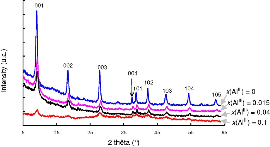
XRD patterns of Al-substituted hydroxysulphate green rust samples that contain increasing amount of aluminium.
Diffractogrammes de rayons X pour des échantillons de rouille verte sulfatée substituée aluminium.

Mössbauer spectra of hydroxysulphate green rust (a) and Al-substituted hydroxysulphate green rust (b).
(a) Spectre Mössbauer de la rouille verte sulfatée, (b) spectre Mössbauer de la rouille verte sulfatée substituée.
Hyperfine parameters of the Mössbauer spectra presented in Fig. 11
Paramètres hyperfins des spectres Mössbauer présentés sur la Fig. 11
| Spectra | Compounds | δ | Δ | FWHM | RA (%) | |
| Fig. 11a | GR( |
D1 | 1.27 | 2.80 | 0.35 | 65 |
| D2 | 0.44 | 0.42 | 0.35 | 35 | ||
| Fig. 11b | Al-GR( |
D1 | 1.27 | 2.84 | 0.34 | 56 |
| D2 | 0.47 | 0.49 | 0.34 | 20 | ||
| D3 | 1.27 | 2.44 | 0.34 | 24 |
A gradual increase of the width of the XRD lines is also observed in Fig. 10. As expected, the size of the hexagonal crystals of Al-GR(
7 Conclusion
The coprecipitation of FeII and FeIII species was studied by using a mass-balance diagram. A direct visualisation of the nature and the relative quantities of the compounds that form is obtained by following simple geometrical rules. In sulphated aqueous medium, the formation of hydroxysulphate green rust {GR(
Acknowledgements
The authors would like to thank Prof. Jean-Pierre Jolivet (‘Université Pierre-et-Marie-Curie’, Paris, France) for fruitful discussion, Dr Jaafard Ghanbaja (‘Université Henri-Poincaré’, Nancy, France) for performing the TEM experiments and Dr Isabelle Bihannic (Laboratoire ‘Environnement Minéralurgie’, INPL, Nancy, France) for the XRD patterns of Al-substituted green rusts.
Vous devez vous connecter pour continuer.
S'authentifier