Multivariate geostatistical simulation by minimising spatial cross-correlation

Babak Sohrabian; Abdullah Erhan Tercan

doi:10.1016/j.crte.2014.01.002

Applied geophysics

Multivariate geostatistical simulation by minimising spatial cross-correlation

Babak Sohrabian ¹ ; Abdullah Erhan Tercan ¹

¹ Hacettepe University, Department of Mining Engineering, 06800 Beytepe, Ankara, Turkey

Comptes Rendus. Géoscience, Volume 346 (2014) no. 3-4, pp. 64-74.

Résumé

Joint simulation of attributes in multivariate geostatistics can be achieved by transforming spatially correlated variables into independent factors. In this study, a new approach for this transformation, Minimum Spatial Cross-correlation (MSC) method, is suggested. The method is based on minimising the sum of squares of cross-variograms at different distances. In the approach, the problem in higher space (N × N) is reduced to $N \times (N - 1) / 2$ problems in the two-dimensional space and the reduced problem is solved iteratively using Gradient Descent Algorithm. The method is applied to the joint simulation of a set of multivariate data in a marble quarry and the results are compared with Minimum/Maximum Autocorrelation Factors (MAF) method.

Métadonnées

Reçu le : 2014-01-09
Accepté le : 2014-01-16
Publié le : 2014-03-01

DOI : 10.1016/j.crte.2014.01.002

Mots clés : Joint simulation, MAF, Multivariate geostatistics, Orthogonalization, Spatial correlation

Affiliations des auteurs :

Babak Sohrabian ¹ ; Abdullah Erhan Tercan ¹

¹ Hacettepe University, Department of Mining Engineering, 06800 Beytepe, Ankara, Turkey

@article{CRGEOS_2014__346_3-4_64_0,
     author = {Babak Sohrabian and Abdullah Erhan Tercan},
     title = {Multivariate geostatistical simulation by minimising spatial cross-correlation},
     journal = {Comptes Rendus. G\'eoscience},
     pages = {64--74},
     publisher = {Elsevier},
     volume = {346},
     number = {3-4},
     year = {2014},
     doi = {10.1016/j.crte.2014.01.002},
     language = {en},
}

TY  - JOUR
AU  - Babak Sohrabian
AU  - Abdullah Erhan Tercan
TI  - Multivariate geostatistical simulation by minimising spatial cross-correlation
JO  - Comptes Rendus. Géoscience
PY  - 2014
SP  - 64
EP  - 74
VL  - 346
IS  - 3-4
PB  - Elsevier
DO  - 10.1016/j.crte.2014.01.002
LA  - en
ID  - CRGEOS_2014__346_3-4_64_0
ER  -

%0 Journal Article
%A Babak Sohrabian
%A Abdullah Erhan Tercan
%T Multivariate geostatistical simulation by minimising spatial cross-correlation
%J Comptes Rendus. Géoscience
%D 2014
%P 64-74
%V 346
%N 3-4
%I Elsevier
%R 10.1016/j.crte.2014.01.002
%G en
%F CRGEOS_2014__346_3-4_64_0

Babak Sohrabian; Abdullah Erhan Tercan. Multivariate geostatistical simulation by minimising spatial cross-correlation. Comptes Rendus. Géoscience, Volume 346 (2014) no. 3-4, pp. 64-74. doi : 10.1016/j.crte.2014.01.002. https://comptes-rendus.academie-sciences.fr/geoscience/articles/10.1016/j.crte.2014.01.002/

Version originale du texte intégral

1 Introduction

Linear transformation of spatially correlated variables into uncorrelated factors has been one of the most challenging issues in mining engineering and earth sciences. In this direction, several methods have been introduced by researchers. Xie et al. (1995) and Tercan (1999) used simultaneous diagonalisation in finding approximately uncorrelated factors at several lag distances by simultaneously diagonalising a set of variogram matrices. Switzer and Green (1984) developed the method of Minimum/Maximum Autocorrelation Factors (MAF) for the objective of separating signals from noise in multivariate imagery observations. The method is first introduced to geostatistical community by Desbarats and Dimitrakopoulos (2000) in the context of multivariate geostatistical simulation of pore-size distributions.

Fonseca and Dimitrakopoulos (2003) used MAF method for assessing risks in grade-tonnage curves in a complex copper deposit. Boucher and Dimitrakopoulos (2009) presented a method for the conditional block simulation of a non-Gaussian vector random field. They, first, orthogonalised a vector random function with MAF method and then used LU simulation to generate possible realizations. Rondon (2011) discussed the joint simulation of spatially cross-correlated variables using MAF factors in detail and gave some examples.

MAF is basically a two-stage principal component analysis applied to variance–covariance matrices at short and long lag distances. Goovaerts (1993) proves that in the presence of a two-structure linear model of co-regionalization (2SLMC), the factors are spatially uncorrelated. But the assumption of a 2SLMC is not reasonable for most of real data sets and also an extension of MAF to more than two distinct structure matrices is not possible (Vargas-Guzmán and Dimitrakopoulos, 2003). In the case where fitting a 2SLMC is not possible, a data-driven version of MAF method can be used (Desbarats and Dimitrakopoulos, 2000; Tercan, 1999; Sohrabian and Ozcelik, 2012a). In this approach, the variance–covariance matrices are calculated directly from the data set.

There are also some studies that use the independency property of the generated factors. For example, Sohrabian and Ozcelik (2012b) introduce Independent Component Analysis (ICA) to transform spatially correlated attributes of an andesite quarry into independent factors. Then they estimated each factor independently and back-transformed the results into the real data space to determine exploitable blocks. Tercan and Sohrabian (2013) used independent component analysis in joint simulation of some quality attributes of a lignite deposit.

Goovaerts (1993) proves that in the general case, it is impossible to find factors that are exactly uncorrelated at all lag distances. When spatially uncorrelated factors cannot be produced, one looks for algorithms that produce approximately uncorrelated factors. For that, Mueller and Ferreira (2012) used Uniformly Weighted Exhaustive Diagonalization with Gauss iterations (U-WEDGE), introduced by Tichavsky and Yeredor (2009), for joint simulation of a multivariate data set from an iron deposit. In their case study, Mueller and Ferreira (2012) show that the U-WEDGE algorithm performs better than MAF.

In the present study, Minimum Spatial Cross-Correlation (MSC) method is introduced for generating approximately uncorrelated factors. It aims to minimise cross-variance matrices at different lag distances using the gradient descent algorithm. In this method the de-correlation problem is reduced to the solution of a sequence of 2 by 2 problems. Against other blind source separation algorithms such as U-WEDGE and ICA which generally work in high-dimensional spaces and try to solve the problem by choosing N × N initial matrices the MSC method is more convenient. In addition, ICA and U-WEDGE algorithms are sensitive to the choice of the initial matrices so that several applications of these algorithms do not converge to the same result (Hyvarinen et al., 2001). But, the MSC method approximately converges to the same result and this can be considered as an advantage over methods that directly solve N × N optimization problems.

The outline of the paper is as follows: the second section describes multivariate random field model. The third section explains the theory of MSC. The method is presented in 2D and then is generalized into an N-dimensional space. In the fourth section the method is applied to joint simulation of multivariate data obtained from an andesite quarry and the efficiency of the method in generating spatially orthogonalised factors is measured and compared to that of MAF method. Then MSC and MAF factors are used to simulate some attributes of a marble quarry. The last section includes the conclusions.

2 The multivariate random field

Let $Z (u) = [Z_{1} (u), Z_{2} (u), ..., Z_{N} (u)]$ be an N-dimensional stationary random field with zero mean and unit variance. In this multivariate case, the variogram matrix is given by

Γ_{Z} (h) = \frac{1}{2} E [(Z (u + h) - Z (u)) {(Z (u + h) - Z (u))}^{T}]

(1)

The variogram matrix depends only on the lag distance h, assuming that correlations vanish as $h \to \infty$ . In the presence of spatial cross-correlation, each variable should be simulated by considering the cross-correlations. In such cases, the traditional method is co-simulation, but it is impractical and time consuming due to difficulties arising from the fitting of a valid model of coregionalisation and the solving of large cokriging systems (Goovaerts, 1993). To ease multivariate simulation, Z(u) can be transformed into spatially uncorrelated factors F(u) in such way that

F (u) = Z (u) W

(2)

where W is an orthogonal transformation matrix. Then each factor

F_{1}, F_{2}, ..., F_{N},

can be simulated separately and simulated factors can be back-transformed into the original space. This is a linear transformation that can remove linear correlations of variables and in the presence of non-linear correlations among variables it cannot be helpful. The transformation process results in factors which should be simulated by using one of the geostatistical methods for which stationary assumption holds. We assume that before running MSC the multivariate data are whitened with principal component analysis. By using principal component analysis, we guarantee the orthogonality of the produced factors. Orthogonal factors can be parameterised by half the parameters which are needed in any arbitrary matrix. Whitening also restricts the possible results to a unit circle (Hyvarinen et al., 2001).

3 MSC Method

Researchers have proposed various methods for generating spatially orthogonal factors. Some criteria have also been introduced to measure how well these methods orthogonalise the variogram matrices at different lag distances. For example, Tercan (1999) proposed the following measure:

τ (h) = \frac{φ (h)}{ξ (h)}, |h| > 0

(3)

where

φ (h) = \sum_{k = 1}^{N} \sum_{k < j}^{N} |γ_{F} (h; k, j)|

and

ξ (h) = \sum_{k = 1}^{N} γ_{F} (h; k, k)

. This measure compares the sum of off-diagonal elements of the factor variogram matrix

Γ_{Z} (h)

to the sum of its diagonal elements for each lag distance h. It is used by Rondon (2011) and Mueller and Ferreira (2012) to compare various factorization algorithms. Efficient factorization algorithms would produce

τ (h)

as close as possible to zero at each lag distance. This measure can also be considered as an optimization criterion in producing the desired factors.

While developing our method in deriving spatially uncorrelated factors, we will consider Eq. 3, proving that $ξ (h)$ is constant (see Appendix A for a proof). Therefore it suffices to minimize the sum of $φ (h)$ values at various lag distances. In the following section, a simple method based on the gradient descent algorithm is presented for iteratively minimizing the $φ$ value.

φ = \sum_{i = 1}^{l} \sum_{k = 1}^{N} \sum_{k < j}^{N} |γ_{F} (h_{i}; k, j)|, |h| > 0

(4)

In Eq. 4, l denotes the number of lags that are considered in the calculations. The number of lags depends on the smallest distance that the experimental variograms are calculated and also on the maximum range of the auto or cross-variograms of variables. The number of lags can be chosen by dividing the maximum range of variograms by the average sampling distance.

Another issue is unequal sampling, which affects the calculation of cross-variograms. In case of partial heterotopy where some variables share some sample locations, it is advisable to infer the cross-variogram model on the basis of the isotopic subset of the data (Wackernagel, 2003). This is known as complete-case analysis. The method suggested in this study works for complete case data. However, this approach reduces the sample size and results in loss of information due to discarding incomplete samples. This can cause loss of precision and potentially bias when the complete cases are not a random sample of the population (Little and Rubin, 2002). Instead, imputation methods can be used to supply missing observations to complete a data set. The approaches to imputing vary from the simplest form, taking an average of nearby simple values, to complicated ones, for example multiple imputation. More detail on imputing can be found in Little and Rubin (2002).

In minimization problems, the derivatives of functions are used widely. It is known that the absolute value of functions may not be differentiable at some points in their domains. We work with whitened data with cross-variograms lying between–1 and 1, so that $|γ_{F} (h_{i}; k, j)|$ can be replaced by ${(γ_{F} (h_{i}; k, j))}^{2}$ without changing in the directions that minimize Eq. 4. Therefore, the objective function takes the following form:

φ = \sum_{i = 1}^{l} \sum_{k = 1}^{N} \sum_{k < j}^{N} {(γ_{F} (h_{i}; k, j))}^{2}, |h| > 0

(5)

In practice, to minimize Eq. 5, we would start from some vector w, compute the direction in which the $φ$ value of new factors F=ZW is growing most rapidly, based on the available samples of spatially correlated variables and then move the vector w in the opposite direction.

3.1 Gradient descent algorithm

This section includes a short explanation of the algorithm. Let f(x) with $x \in ℝ^{n}$ , be a differentiable scalar field. We want to find its minimum. Then the gradient $\partial f (x) / \partial (x)$ at location x represents a direction where the function increases and $- \partial f (x) / \partial (x)$ is usually called the steepest descent direction. For finding the minimum of f(x), the gradient descent algorithm starts from an initial point x₁, then iteratively takes a step along the steepest descent direction, optionally scaled by a step length, until convergence. Gradient descent is popular for very large-scale optimization problems because it is easy to implement and its iterations are cheap.

The algorithm typically converges to a local minimum, but in the presence of only one saddle point it gives a global minimum. If $x_{1} \in ℝ^{n}$ is a starting point, $α$ a step length, $ε$ a tolerance value or constraint, and f(x) an objective function, then the algorithm can be given as follows:

1. start iteration $t = 1$
2. $x_{t} \leftarrow x_{t - 1} - α \frac{\partial f (x)}{\partial (x)}$
3. if f(x_t) > f(x_t-1) then $α \leftarrow \frac{α}{2}$
4. if $abs (Δ x) > ε$ go to step 2
5. end

The objective function of our optimization problem is presented in Eq. 5. In this study, an N × N optimization problem will be replaced by a set of two-dimensional problems, so that, at first, we assume the simplest case of two spatially cross-correlated variables. In Eq. 5, the aim is to find a transformation matrix, W, which gives factors with the lowest spatial cross-correlation. The columns of matrix W, denoted by w, give the directions of the factors that we are looking for. To restrict the number of possible w vectors, a whitening process is performed by using principal component analysis therefore the mean and variance of Z become 0 and 1, respectively. The optimization problem is now reduced to a unit circle and we search for a vector w so that the linear combination ZW has a minimum $φ$ value. For this two-dimensional case, the point on the unit sphere can be parameterized by the angle $θ$ that the corresponding vector w makes with the horizontal axis. The function $φ$ is periodic, with a period equal to $π / 2$ rad, and the vector w gives the direction of the first factor. The direction of the second factor is perpendicular to that of the first one.

3.2 Minimizing $φ$ value between two variables using gradient descent algorithm

Assume that the experimental semivariogram matrix for h_i is given as follows:

Γ_{Z} (h_{i}) = [\begin{array}{c} γ_{11} (h_{i}) & γ_{12} (h_{i}) \\ γ_{12} (h_{i}) & γ_{22} (h_{i}) \end{array}]

(6)

The objective is to find a 2 × 2 transformation matrix W

W = [\begin{array}{c} \cos θ & - \sin θ \\ \sin θ & \cos θ \end{array}]

(7)

which generates the factors with minimum cross-correlation. The variogram matrix of the factors can then be written as follows:

Γ_{F} (h_{i}) = W {(θ)}^{T} Γ_{Z} (h_{i}) W (θ) = [\begin{array}{c} cos θ & \sin θ \\ - \sin θ & cos θ \end{array}] [\begin{array}{c} γ_{11} (h_{i}) & γ_{12} (h_{i}) \\ γ_{12} (h_{i}) & γ_{22} (h_{i}) \end{array}] [\begin{array}{c} \cos θ & - \sin θ \\ \sin θ & \cos θ \end{array}] = [\begin{array}{c} {cos}^{2} θ γ_{11} (h_{i}) + \sin^{2} θ γ_{22} (h_{i}) + 2 \cos θ \sin θ γ_{12} (h_{i}) & \cos θ \sin θ (γ_{22} (h_{i}) - γ_{11} (h_{i})) + (\cos^{2} θ - \sin^{2} θ) γ_{12} (h_{i}) \\ cos θ \sin θ (γ_{22} (h_{i}) - γ_{11} (h_{i})) + (\cos^{2} θ - \sin^{2} θ) γ_{12} (h_{i}) & \cos^{2} θ γ_{22} (h_{i}) + \sin^{2} θ γ_{11} (h_{i}) - 2 \cos θ \sin θ γ_{12} (h_{i}) \end{array}]

(8)

and in that case the expression to be minimised is:

φ (θ) = \sum_{i = 1}^{l} {[γ_{F_{1} F_{2}} (h_{i})]}^{2} = \sum_{i = 1}^{l} {[\cos θ \sin θ (γ_{22} (h_{i}) - γ_{11} (h_{i})) + (\cos^{2} θ - \sin^{2} θ) γ_{12} (h_{i})]}^{2}

(9)

Eq. 9 has only one parameter $(θ)$ and we can use gradient descent (Battiti, 1992; Hyvarinen et al., 2001) to minimize it iteratively. For minimization of $φ$ , we start from an initial point, $θ$ , compute the gradient of $φ$ at this point and move in the direction of negative gradient or the steepest descent by suitable distance. Repeat the same procedure at the new point, and so on. The derivative of $φ (θ)$ with respect to $θ$ is:

\begin{array}{l} \frac{\partial φ (θ)}{\partial θ} = \frac{\partial \sum_{i = 1}^{l} {(γ_{F_{1} F_{2}} (h_{i}))}^{2}}{\partial θ} = \\ \sum_{i = 1}^{l} [(\cos^{3} θ \sin θ - \sin^{3} θ \cos θ) (2 K_{i}^{2} - 8 γ_{12}^{2} (h_{i})) + 2 K_{i} (\cos^{4} θ + \sin^{4} θ - 6 \times \cos^{2} θ \sin^{2} θ) γ_{12} (h_{i})] \end{array}

(10)

where

K_{i} = γ_{22} (h_{i}) - γ_{11} (h_{i})

(Appendix A).

3.3 Applying the algorithm to an N–dimensional case

Blind source separation methods such as independent component algorithms use N × N matrices and their first- and second-order derivatives, which are difficult to manage (Sohrabian and Ozcelik, 2012b; Tercan and Sohrabian, 2013). On the other hand, the new developed algorithm is simple as you only need to solve $N \times (N - 1) / 2$ one-dimensional problems, while the actual matrices are still N by N. The N × N space is divided into $N \times (N - 1) / 2$ two-dimensional spaces and the previous algorithm is run for each 2-D space where the related axes are rotated to renew the factors, and the algorithm is set to work for the remaining 2-D spaces. In case of N × N space, the problem is simplified to the calculation of $N \times (N - 1) / 2$ rotation angles. Then, the final transformation matrix is calculated as follows:

\begin{array}{l} A_{MSC} = \prod_{i = 1}^{N \times (N - 1) / 2} A (θ_{i}) = A (θ_{1}) \times A (θ_{2}) \times ... \times A (θ_{N \times \frac{N - 1}{2}}) \\ = [\begin{array}{c} \cos θ_{1} & - \sin θ_{1} & 0 \dots 0 & 0 \\ \sin θ_{1} & \cos θ_{1} & 0 \dots 0 & 0 \\ ⋮_{0}^{0} & ⋮_{0}^{0} & {⋮ ⋱ ⋮}_{0 \dots 1}^{1 \dots 0} & ⋮_{0}^{0} \\ 0 & 0 & 0 \dots 0 & 1 \end{array}] \times [\begin{array}{c} \cos θ_{2} & 0 & - \sin θ_{2} & 0 \dots 0 \\ 0 & 1 & 0 & 0 \dots 0 \\ \sin θ_{2} & 0 & \cos θ_{2} & 0 \dots 0 \\ ⋮_{0}^{0} & ⋮_{0}^{0} & ⋮_{0}^{0} & {⋮ ⋱ ⋮}_{0 \dots 1}^{1 \dots 0} \end{array}] \times ... \\ \times [\begin{array}{c} 1 & 0 \dots 0 & 0 & 0 \\ ⋮_{0}^{0} & {⋮ ⋱ ⋮}_{0 \dots 1}^{1 \dots 0} & ⋮_{0}^{0} & ⋮_{0}^{0} \\ 0 & 0 \dots 0 & \cos θ_{N \times \frac{N - 1}{2}} & - \sin θ_{N \times \frac{N - 1}{2}} \\ 0 & 0 \dots 0 & \sin θ_{N \times \frac{N - 1}{2}} & \cos θ_{N \times \frac{N - 1}{2}} \end{array}] \end{array}

(11)

This technique is applied to an andesite deposit containing four variables to illustrate how $τ (h)$ decreases after each 2-D rotation (Fig. 1). Considering the maximum range of auto and cross-variograms and the average distance of sample locations, we chose five variogram matrices at distances 20 m, 40 m, 60 m, 80 m and 100 m. The magnitude of derivative obtained from iteration was too small and therefore the initial value for $α$ was taken to be 5000. The value of $α$ was divided by 2 for five times as getting closer to the minimum point. Fig. 1 shows that, after each 2-dimensional transformation and renewing factors, the $τ (h)$ value decreases gradually from the whitened components to the MSC factors.

Fig. 1
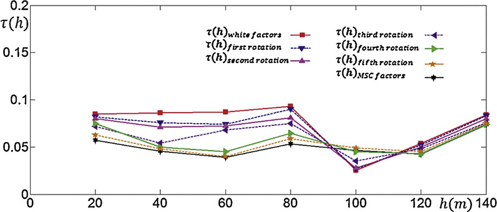
(Colour online) Decrease in $τ (h)$ value as iteration progresses in 2-D spaces. For example shows $τ (h)$ values of factors obtained after first rotation in 2-D space of first and second factors.

4 Case study

The study area is an andesite quarry located in the Çubuk district, 60 km north-east of Ankara, Turkey. In the area, a total of 108 samples at 20-m regular intervals were collected and the samples were tested for Uniaxial Compressive Strength (UCS), Tensile Strength (TS), Elasticity Modulus (EM) and Los Angeles abrasion for 500 revolutions (Los 500) according to Turkish standards (TSE, 1987). The mechanical properties are tested on core samples with the same size. Therefore the variables considered in the study can be said to be additive. Among these variables, EM and TS are positively skewed and Los 500 is strongly negatively skewed. The UCS is the only attribute with a symmetric distribution (not shown here). Table 1 gives summary statistics for each variable and correlation coefficients between them. Correlation coefficients are relatively high with absolute values more than 0.8. The highest correlation coefficient occurs between Los 500 and TS and then UCS and TS.

Variable	Minimum	Mean	Maximum	Skewness	Variance
EM	7.80	14.20	28.70	1.09	23.16
TS	5.09	8.76	13.45	0.32	5.30
UCS	20.00	63.35	105.00	0.00	375.07
Los 500	11.20	14.31	16.20	–0.63	1.48
		Correlation coefficient matrix of variables
		EM	TS	UCS	Los 500
	EM	1	0.82	0.80	–0.82
	TS	0.82	1	0.94	–0.94
	UCS	0.80	0.94	1	–0.88
	Los 500	–0.82	–0.94	–0.88	1

4.1 Transformations

MSC method was run by considering the sum of cross-variograms at five lag distances. Lag distance and lag tolerance were chosen as 20 m and 10 m, respectively. Prior to running MSC method, a whitening process was performed by using PCA. Whitening process and MSC transformation were done using T_whitening and A_MSC matrices, respectively:

\begin{array}{l} T_{whitening} = [\begin{array}{c} 0.01 & 0.04 & 0.09 & 0.12 \\ 0.12 & 0.27 & - 0.02 & - 1.81 \\ 0.05 & - 0.37 & 0.06 & - 0.04 \\ - 0.22 & - 0.29 & 1.76 & - 1.76 \end{array}], \\ A_{MSC} = [\begin{array}{c} - 0.14 & 0.76 & 0.17 & - 0.62 \\ - 0.57 & - 0.35 & 0.74 & - 0.08 \\ - 0.63 & - 0.25 & - 0.65 & - 0.34 \\ 0.50 & - 0.5 & 0.07 & - 0.71 \end{array}] \end{array}

Overall transformation matrix = T_{whitening} \times A_{MSC} = [\begin{array}{c} - 0.03 & 0.09 & - 0.03 & - 0.13 \\ - 1.07 & 0.90 & 0.11 & 1.19 \\ 0.15 & 0.17 & - 0.31 & 0.01 \\ - 1.80 & 0.37 & - 1.53 & 0.80 \end{array}]

For MAF approach, auto and cross-variograms of standardised variables were calculated at two lag distances equal to 28 and 100 m. Then, the overall transformation matrix from original data to MAF factors was obtained:

A_{MAF} = [\begin{array}{c} 0.09 & - 0.06 & 0.02 & - 0.13 \\ 0.05 & - 0.19 & - 0.24 & 1.77 \\ 0.09 & 0.34 & - 0.12 & - 0.03 \\ 1.85 & 0.01 & 0.18 & 1.22 \end{array}]

The MSC and MAF factors were produced by multiplying the transforming matrices by the data matrix. Fig. 2 shows the cross-variograms of factors obtained by these methods. Fig. 2 also compares the efficiency of orthogonalization methods using $τ (h)$ measure. It is obvious that the cross-variograms of the MSC factors are in a tighter interval than those of MAF factors. Considering $τ (h)$ values, the MSC method seems to be more efficient than MAF method in producing orthogonalised factors at most lag distances but 100 m.

Fig. 2
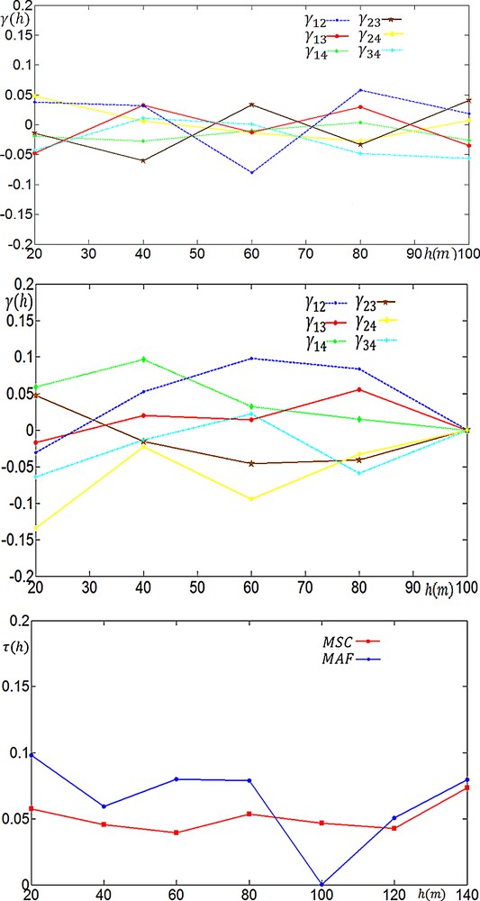
(Colour online) Cross-variograms of factors obtained by MSC (top left) and MAF (top right) methods and their orthogonalization efficiency plot (bottom).

4.2 Simulations

By running the Jarque–Bera test of normality at the 5% significance level, it can be said that all factors but MAF3 have a normal distribution. Experimental variograms of MSC and MAF factors are calculated and shown together with the fitted models and model parameters (Fig. 3). The model variograms of all factors consist of pure nugget and of one spherical scheme. All factors have isotropic variogram models except the third MSC factor. For each factor, 100 realizations were generated separately by considering the direct sequential simulation algorithm introduced by Oz et al., 2003. Most factors show normal distribution so that they can be simulated by the direct sequential simulation method without any normal scores transformation. The simulated realizations were then back-transformed into the real data space. For simulation, a 5 × 5 regular grid containing 1911 nodes was used.

Fig. 3
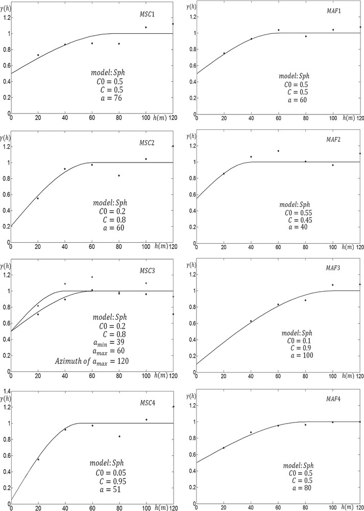
(Colour online) Auto-variograms of MSC and MAF factors together with the fitted models (black solid line) and model parameters.

4.3 Comparison of the simulation results

To compare MSC and MAF simulations, some tests were carried out. For this purpose, the following criteria are considered: reproduction of summary statistics, cumulative histograms, correlation coefficients and auto/cross-variograms.

The mean and variance values of 100 realizations obtained from both simulation methods are shown in Fig. 4. Practically, there is no noticeable difference between mean values of MSC and MAF realizations. Compared to the variance of actual values, the variance of MAF realizations is high, while the variance of MSC realizations is low. Fig. 5 shows the cumulative histograms of realizations obtained from MSC and MAF simulations. It can be said that reproduction of CDF is acceptable for both methods.

Fig. 4
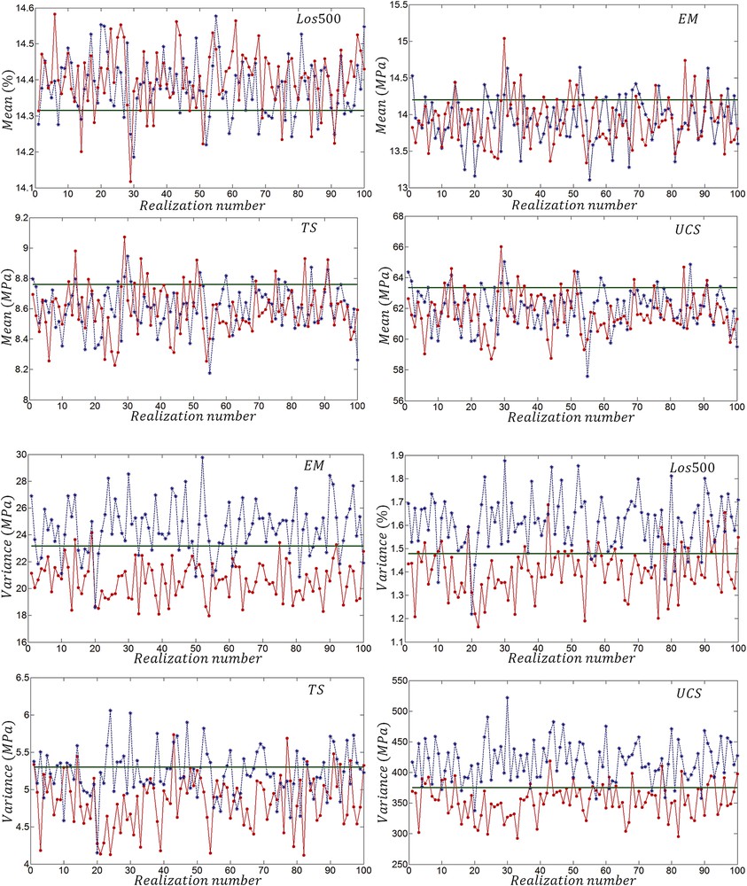
(Colour online) Comparison of the mean and variance of variables (green straight line) with simulated realizations obtained using MSC () and MAF () factors.

Fig. 5
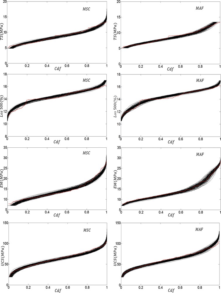
(Colour online) Cumulative distribution functions for one hundred realizations for each attribute obtained using the MSC and MAF simulation methods. Solid red lines demonstrate the cumulative distribution function of the original variables.

The next test consists in comparing the correlation coefficients of simulations to those of real data. The reproduction of sample correlations is perfect for MSC simulations and reasonable for MAF simulations (Fig. 6). In general, for each attribute, the mean value of correlation coefficients of MSC simulations is closer to the sample correlation coefficient.

Fig. 6
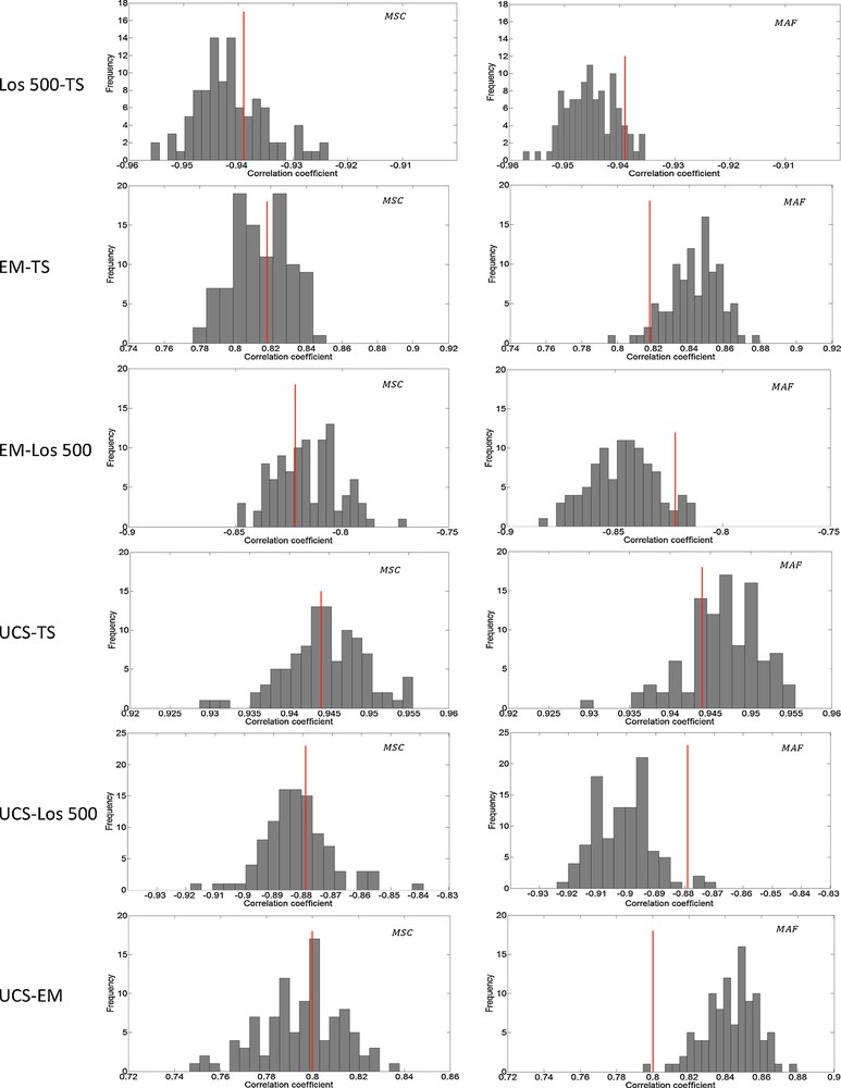
Histogram of simulation correlation coefficients together with aimed values (red solid line) (For interpretation of the references to color in this figure, the reader is referred to the web version of this article).

The experimental auto and cross-variograms of 100 realizations for both methods are shown in Fig. 7. The experimental variograms for MSC simulation change in a narrow interval compared to the experimental variograms of MAF simulation. This is an expected result when we consider the variances of the realizations for both methods as shown in Fig. 4. In average, the sample variograms are well produced by MSC over MAF. In addition, MSC reproduces short-range variability better than MAF.

Fig. 7
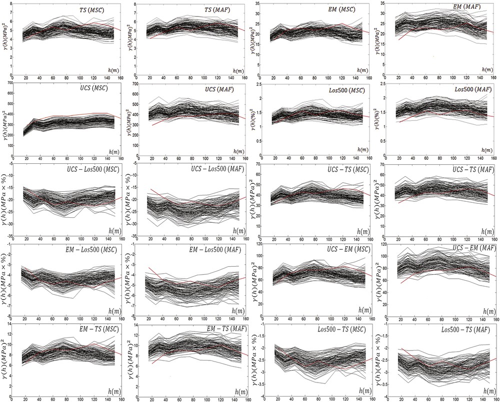
Auto and cross-variograms (black solid lines) of simulation results together with target variograms (red solid line). (For interpretation of the references to colour in this figure, the reader is referred to the web version of this article).

5 Conclusions

In this paper, a novel method is presented for spatially orthogonalization of multivariate data. Then, the results of joint simulations obtained by this method are compared to MAF simulations. MSC simulation method shows better performance over MAF. At most lag distances, the factors generated by MSC method have lower $τ$ values than MAF factors so that they are spatially more uncorrelated than factors obtained by MAF method.

The case study shows that the reproduction of target statistics for MSC and MAF simulations is acceptable. The methods produce practically similar average values. MSC produces the simulated realizations with low variances, while MAF realizations show high variances. The CDF reconstruction of simulated attributes is acceptable for both methods. However, the reproduction of target correlation coefficients is good for MSC method and reasonable for MAF simulation. Also, MSC simulations reproduce auto and cross-variograms better than MAF simulations. In particular, the short-range variability is well produced in MSC.

Minimization of cross-variograms is not the only criterion to use. Some other criteria can also be defined. For example, a new measure of spatial independency rather than spatial uncorrelatedness can be introduced. In addition, the MSC criterion based on the minimization of cross-variograms at different distances assumes that each distance is equally weighted. One can however consider different weights for each distance. MSC algorithm cannot handle non-linear correlations among variables since it uses linear transformations. Therefore, the method should be developed further in order to consider non-linear correlations.

Acknowledgement

This study is supported by the Scientific and Technical Research Council of Turkey (TUBITAK) under Grant 111M218.

Appendix A

Proof: Suppose that the number of variables is equal to 2. This can be easily generalized to N. $ξ_{Z} (h_{i}) = \sum_{k = 1}^{2} γ_{Z} (h_{i}; k, k) = γ_{11} (h_{i}) + γ_{22} (h_{i}), \in h_{i}$ is constant:

$ξ_{Z} (h_{i}) = \sum_{k = 1}^{2} γ_{Z} (h_{i}; k, k) = γ_{11} (h_{i}) + γ_{22} (h_{i}), \in h_{i}$ , $\in h_{i}$ for the whitened data and also

\begin{array}{l} ξ_{F} (h_{i}) = \sum_{k = 1}^{2} γ_{F} (h_{i}; k, k) \\ = \cos^{2} θ γ_{11} (h_{i}) + \sin^{2} θ γ_{22} (h_{i}) + 2 \cos θ \sin θ γ_{12} (h_{i}) + \cos^{2} θ γ_{22} (h_{i}) + \sin^{2} θ γ_{11} (h_{i}) - 2 \cos θ \sin θ γ_{12} (h_{i}) \\ = (\cos^{2} θ + \sin^{2} θ) γ_{11} (h_{i}) + (\cos^{2} θ + \sin^{2} θ) γ_{22} (h_{i}) = γ_{11} (h_{i}) + γ_{22} (h_{i}) \end{array}

for the MSC factors.

The derivative of $φ (θ)$ with respect to $θ$ can be given as follows:

\begin{array}{l} \frac{\partial φ (θ)}{\partial θ} = \frac{\partial {\sum_{i = 1}^{l} (γ_{F_{1} F_{2}} (h_{i}))}^{2}}{\partial θ} \\ = \sum_{i = 1}^{l} [(\cos^{3} θ \sin θ - \sin^{3} θ \cos θ) (2 K_{i}^{2} - 8 γ_{12}^{2} (h_{i})) + 2 K_{i} (\cos^{4} θ + \sin^{4} θ - 6 K_{i} \cos^{2} θ \sin^{2} θ) γ_{12} (h_{i})] \end{array}

The expansion of $γ_{F_{1} F_{2}} (h_{i})$ in terms of $θ$ is:

γ_{F_{1} F_{2}} (h_{i}) = K_{i} \cos θ \sin θ + (\cos^{2} θ - \sin^{2} θ) γ_{12} (h_{i})

with

K_{i} = γ_{22} (h_{i}) - γ_{11} (h_{i})

The derivative of $γ_{F_{1} F_{2}} (h_{i})$ with respect to $θ$ is as follows:

\frac{\partial {γ_{F_{1} F_{2}} (h_{i})}}{\partial θ} = K_{i} (\cos^{2} θ - \sin^{2} θ) - 4 \cos θ \sin θ γ_{12} (h_{i})

Then

\frac{\partial φ (θ)}{\partial θ} = \frac{\partial \sum_{i = 1}^{l} {(γ_{F_{1} F_{2}} (h_{i}))}^{2}}{\partial θ}

\begin{array}{l} = 2 \times \sum_{i = 1}^{l} \frac{\partial {γ_{F_{1} F_{2}} (h_{i})}}{\partial θ} \times γ_{F_{1} F_{2}} (h_{i}) \\ = 2 \sum_{i = 1}^{l} [K_{i} (\cos^{2} θ - \sin^{2} θ) - 4 \cos θ \sin θ γ_{12} (h_{i})] \cdot [K_{i} \cos θ \sin θ + (\cos^{2} θ - \sin^{2} θ) γ_{12} (h_{i})] \\ = \sum_{i = 1}^{l} [2 K_{i}^{2} (\cos^{3} θ \sin θ - \sin^{3} θ \cos θ) + 2 K_{i} {(\cos^{2} θ - \sin^{2} θ)}^{2} γ_{12} (h_{i}) - 8 K_{i} \cos^{2} θ \sin^{2} θ γ_{12} (h_{i}) - 8 (\cos^{3} θ \sin θ - \sin^{3} θ \cos θ) γ_{12}^{2} (h_{i})] \end{array}

= \sum_{i = 1}^{l} [(\cos^{3} θ \sin θ - \sin^{3} θ \cos θ) (2 K_{i}^{2} - 8 γ_{12}^{2} (h_{i})) + 2 K_{i} (\cos^{4} θ + \sin^{4} θ - 6 \times \cos^{2} θ \sin^{2} θ) γ_{12} (h_{i})]

Bibliographie

[Battiti, 1992] R. Battiti First-and second-order methods for learning: between steepest descent and Newton's method, Neural computation MIT Press, 1992

[Boucher and Dimitrakopoulos, 2009] A. Boucher; R. Dimitrakopoulos Block-support simulation of multiple correlated variables, Math. Geosci., Volume 41 (2009) no. 2, pp. 215-237

[Desbarats and Dimitrakopoulos, 2000] A. Desbarats; R. Dimitrakopoulos Geostatistical simulation of regionalized pore-size distribution using min/max autocorrelation factors, Math. Geol., Volume 32 (2000) no. 8, pp. 919-942

[Fonseca and Dimitrakopoulos, 2003] M. Fonseca; R. Dimitrakopoulos, Application of computers and operations research in the mineral industries, South African Institute of Mining and Metallurgy (2003), pp. 373-382

[Goovaerts, 1993] P. Goovaerts Spatial orthogonality of the principal components computed from coregionalized variables, Math. Geol., Volume 25 (1993) no. 3, pp. 281-302

[Hyvarinen et al., 2001] A. Hyvarinen; J. Karhunen; E. Oja Independent Component Analysis, John Wiley & Sons, 2001 (481 p.)

[Little and Rubin, 2002] R.J.A. Little; D.B. Rubin Statistical analysis with missing data, John Wiley & Sons, Hoboken, 2002

[Mueller and Ferreira, 2012] U.A. Mueller; J. Ferreira The U-WEDGE Transformation Method for Multivariate Geostatistical Simulation, Math. Geosci. (2012) | DOI

[Oz et al., 2003] B. Oz; C.V. Deutsch; T.T. Tran; Y. Xie DSSIM-HR: A FORTRAN 90 program for direct sequential simulation with histogram reproduction, Comput. Geosci., Volume 29 (2003) no. 1, pp. 39-51

[Rondon, 2011] O. Rondon Teaching Aid: Minimum/Maximum Autocorrelation Factors for Joint Simulation of Attributes, Math. Geosci. (2011) | DOI

[Sohrabian and Ozcelik, 2012a] B. Sohrabian; Y. Ozcelik Joint simulation of a building stone deposit using minimum/maximum autocorrelation factors, Construction and Building Materials, Volume 37 (2012), pp. 257-268

[Sohrabian and Ozcelik, 2012b] B. Sohrabian; Y. Ozcelik Determination of exploitable blocks in an andesite quarry using independent component kriging, Int. J. Rock Mech. Mining Sci., Volume 55 (2012), pp. 71-79

[Switzer and Green, 1984] P. Switzer; A. Green Min/max autocorrelation factors for multivariate spatial imaging. Technical report No. 6, Department of Statistics, Stanford University, Stanford, California, 1984

[Tercan, 1999] A.E. Tercan Importance of orthogonalization algorithm in modeling conditional distributions by orthogonal transformed indicator methods, Math. Geol., Volume 31 (1999) no. 2, pp. 155-173

[Tercan and Sohrabian, 2013] A.E. Tercan; B. Sohrabian Multivariate geostatistical simulation of coal quality data by independent components, Int. J. Coal Geol., Volume 112 (2013), pp. 53-66

[Tichavsky and Yeredor, 2009] P. Tichavsky; A. Yeredor Fast approximate joint diagonalization incorporating weight Matrices, IEEE Trans. Signal Process., Volume 57 (2009), pp. 878-891

[TSE, 1987] TSE Methods of Testing for Natural Building Stones (TS 699), TSE Publication, 1987

[Vargas-Guzmán and Dimitrakopoulos, 2003] J. Vargas-Guzmán; R. Dimitrakopoulos Computational properties of min/max autocorrelation factors, Comput. Geosci., Volume 29 (2003) no. 6, pp. 715-723

[Xie et al., 1995] T. Xie; D.E. Myers; A.E. Long Fitting matrix-valued variogram models by simultaneous diagonalization, Part II: application, Math. Geol., Volume 27 (1995) no. 7, pp. 877-888

[Wackernagel, 2003] H. Wackernagel Multivariate Geostatistics: An Introduction with Applications, Springer Verlag, 2003

Commentaires - Politique

Ces articles pourraient vous intéresser

Assessing heterotopic searching strategy in hierarchical cosimulation for modeling the variables with inequality constraints

Sultan Abulkhair; Nasser Madani

C. R. Géos (2021)

Comparing sequential Gaussian and turning bands algorithms for cosimulating grades in multi-element deposits

Shahrokh Paravarzar; Xavier Emery; Nasser Madani

C. R. Géos (2015)

Spatial distribution of pH and organic matter in urban soils and its implications on site-specific land uses in Xuzhou, China

Yingming Mao; Shuxun Sang; Shiqi Liu; ...

C. R. Biol (2014)