Challenges and opportunities in atomistic simulations of glasses: a review

Han Liu; Zhangji Zhao; Qi Zhou; Ruoxia Chen; Kai Yang; Zhe Wang; Longwen Tang; Mathieu Bauchy

doi:10.5802/crgeos.116

Challenges and opportunities in atomistic simulations of glasses: a review
[Défis et opportunités en simulations atomiques de verres : une revue]

Han Liu ¹ ; Zhangji Zhao ¹ ; Qi Zhou ¹ ; Ruoxia Chen ¹ ; Kai Yang ¹ ; Zhe Wang ¹ ; Longwen Tang ¹ ; Mathieu Bauchy ¹

¹ Physics of AmoRphous and Inorganic Solids Laboratory (PARISlab), Department of Civil and Environmental Engineering, University of California, Los Angeles, CA 90095, USA

Comptes Rendus. Géoscience, Volume 354 (2022) no. S1, pp. 35-77.

Résumés

Anglais
Français

Atomistic modeling and simulations have been pivotal in our understanding of the glassy state. Indeed, atomistic modeling offers direct access to the structure and dynamics of atoms in glasses—which is typically hidden from conventional experiments. Simulations also offer a more economical, faster alternative to systematic experiments to decode composition-property relationships and accelerate the discovery of new glasses with desirable properties and functionalities. However, the atomistic modeling of glasses remains plagued by a series of challenges, e.g., high computational cost, limited accessible timescale, lack of accurate interatomic forcefields, etc. These challenges often result in the existence of discrepancies between simulation and experimental data, thereby limiting the predictive power of atomistic modeling. Here, we review recent accomplishments and remaining challenges facing the atomistic modeling of glasses. We discuss future opportunities offered by the seamless integration of simulations, knowledge, experiments, and machine learning in advancing glass modeling to a new era.

La modélisation et simulations atomiques ont joué un rôle important pour notre connaissance de l’état vitreux. En effet, la modélisation atomique offre un accès direct à la structure et dynamique des atomes dans les verres — qui n’est typiquement pas accessible par les techniques expérimentales classiques. Les simulations offrent également une alternative économique et rapide aux expériences systématiques pour décoder les relations composition-propriétés et accélérer la découverte de nouveaux verres offrant des propriétés et fonctionnalités de choix. Cependant, la modélisation atomique des verres reste limitée par une série de défis, par exemple, le coût de calcul élevé, l’échelle de temps accessible limitée, le manque de champs de force interatomiques précis, etc. Ces défis induisent souvent l’existence de divergences entre les résultats simulés et expérimentaux, ce qui limite le pouvoir prédictif de la modélisation atomistique. Dans cette contribution, nous passons en revue les récents progrès et les défis restants auxquels est confrontée la modélisation atomistique des verres. Nous discutons les opportunités futures offertes par les intégrations de simulations, connaissances, données expérimentales et d’intelligence artificielle pour faire avancer la modélisation du verre vers une nouvelle ère.

Métadonnées

Reçu le : 2021-07-30
Révisé le : 2022-02-01
Accepté le : 2022-02-02
Première publication : 2022-05-02
Publié le : 2022-12-01

DOI : 10.5802/crgeos.116

Keywords: Molecular dynamics, Interatomic forcefield, Reserve Monte Carlo, Machine learning, Accelerated simulation, Differentiable programming, Inverse design
Mot clés : dynamique moléculaire, champ de force interatomique, Monte Carlo, machine learning, simulation accélérée, programmation différentiable, design inverse

Affiliations des auteurs :

Han Liu ¹ ; Zhangji Zhao ¹ ; Qi Zhou ¹ ; Ruoxia Chen ¹ ; Kai Yang ¹ ; Zhe Wang ¹ ; Longwen Tang ¹ ; Mathieu Bauchy ¹

¹ Physics of AmoRphous and Inorganic Solids Laboratory (PARISlab), Department of Civil and Environmental Engineering, University of California, Los Angeles, CA 90095, USA

Licence :

CC-BY 4.0

Droits d'auteur : Les auteurs conservent leurs droits

@article{CRGEOS_2022__354_S1_35_0,
     author = {Han Liu and Zhangji Zhao and Qi Zhou and Ruoxia Chen and Kai Yang and Zhe Wang and Longwen Tang and Mathieu Bauchy},
     title = {Challenges and opportunities in atomistic simulations of glasses: a review},
     journal = {Comptes Rendus. G\'eoscience},
     pages = {35--77},
     publisher = {Acad\'emie des sciences, Paris},
     volume = {354},
     number = {S1},
     year = {2022},
     doi = {10.5802/crgeos.116},
     language = {en},
}

TY  - JOUR
AU  - Han Liu
AU  - Zhangji Zhao
AU  - Qi Zhou
AU  - Ruoxia Chen
AU  - Kai Yang
AU  - Zhe Wang
AU  - Longwen Tang
AU  - Mathieu Bauchy
TI  - Challenges and opportunities in atomistic simulations of glasses: a review
JO  - Comptes Rendus. Géoscience
PY  - 2022
SP  - 35
EP  - 77
VL  - 354
IS  - S1
PB  - Académie des sciences, Paris
DO  - 10.5802/crgeos.116
LA  - en
ID  - CRGEOS_2022__354_S1_35_0
ER  -

%0 Journal Article
%A Han Liu
%A Zhangji Zhao
%A Qi Zhou
%A Ruoxia Chen
%A Kai Yang
%A Zhe Wang
%A Longwen Tang
%A Mathieu Bauchy
%T Challenges and opportunities in atomistic simulations of glasses: a review
%J Comptes Rendus. Géoscience
%D 2022
%P 35-77
%V 354
%N S1
%I Académie des sciences, Paris
%R 10.5802/crgeos.116
%G en
%F CRGEOS_2022__354_S1_35_0

Han Liu; Zhangji Zhao; Qi Zhou; Ruoxia Chen; Kai Yang; Zhe Wang; Longwen Tang; Mathieu Bauchy. Challenges and opportunities in atomistic simulations of glasses: a review. Comptes Rendus. Géoscience, Volume 354 (2022) no. S1, pp. 35-77. doi : 10.5802/crgeos.116. https://comptes-rendus.academie-sciences.fr/geoscience/articles/10.5802/crgeos.116/

Version originale du texte intégral (Proposez une traduction )

1. Introduction

As out-of-equilibrium phases, glasses exhibit a complex disordered atomistic structure that can virtually accommodate the entire periodic table [Mauro 2018; Musgraves et al. 2019; Zanotto and Coutinho 2004]. This structural complexity has historically limited our ability to unveil structure–property relationships in glasses [Bapst et al. 2020; Tanaka et al. 2019, 2010], but, in turn, offers a vast design space to discover new glasses with unusual properties [Liu et al. 2019d; Onbaşlı et al. 2018; Ravinder et al. 2020]. Although different experimental protocols have been developed to investigate the nature of the linkages between glass composition, structure, and properties [Almeida and Santos 2015; Kamitsos 2015; Salmon and Zeidler 2015; Youngman 2018], they yield a series of structural fingerprints that are experimentally accessible—e.g., pair distribution function (PDF) computed by diffraction experiments or coordination numbers accessed by nuclear magnetic resonance (NMR) [Fischer et al. 2005; Kroeker 2015; Wright 1988; Youngman 2018]—rather than offering a direct access to the three-dimensional atomic structure itself [Affatigato 2015; Greaves and Sen 2007; Huang et al. 2013; Yang et al. 2021; Zhou et al. 2021]. In that regard, atomistic simulations have become a routine tool to easily access the atomistic structure of glasses [Bauchy 2019; Du 2019; Pedone 2009]—which is otherwise invisible from conventional experiments [Pandey et al. 2016b, a]—and to decipher the physical nature of the linkages between glass structure and properties [Binder and Kob 2011; Massobrio 2015; Onbaşlı and Mauro 2020]. Atomistic simulations of glasses can be broadly divided into two different families, namely, knowledge-based and data-based.

1.1. Physical-knowledge-based simulations

Figure 1.
Schematic illustrating the atomistic simulation of glasses through (i) physical-knowledge-based simulations, e.g., molecular dynamics (MD) simulations [Soules 1990], and (ii) experimental-data-based simulations, e.g., reverse Monte Carlo (RMC) simulations [McGreevy 2001]. Simulations offer a direct access to the atomistic structure of glasses that can be validated by experiments, while, in turn, experiments can offer some fingerprints of the atomistic structure that can be used as simulation constraints. Note that, despite the pronounced difference of timescale between experiments and MD simulations, a direct comparison between MD and experimental data is possible for melts—since the structure and properties of equilibrium liquids and metastable-equilibrium supercooled liquids do not depend on their thermal history [Le Losq et al. 2017].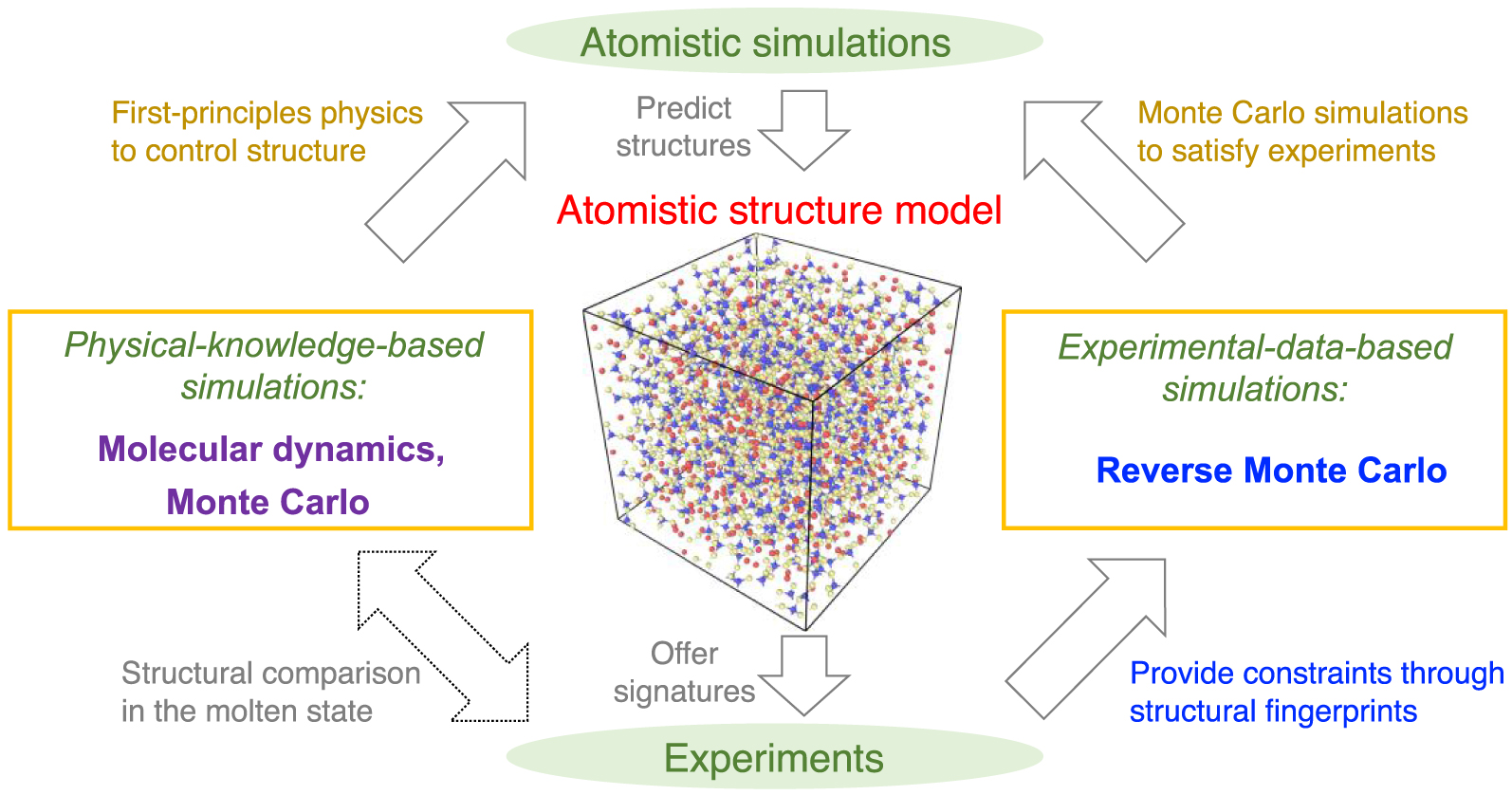

As a primary goal, atomistic simulations aim to reveal the atomistic structure of glasses [Mauro et al. 2016; Takada 2021]. This can be achieved by explicitly simulating the time-dependent formation process of glasses—e.g., melt-quenching [Debenedetti and Stillinger 2001], sol–gel transition [Du et al. 2018], vapor deposition [Wang et al. 2020], irradiation [Krishnan et al. 2017a, b], or annealing [Grigoriev et al. 2016]. Such simulations rely on our knowledge of the physics governing the interaction between atoms, i.e., the interatomic forcefields (see Figure 1) [Massobrio 2015; Mauro et al. 2016; Onbaşlı and Mauro 2020]. In detail, starting from the sole knowledge of first-principles electron interactions [Hohenberg and Kohn 1964; Kohn and Sham 1965], one can compute the interatomic interactions acting in a glass system [Boero et al. 2015; Hafner 2008]. In turn, this interatomic forcefield drives the motions of the atoms as per Newton’s law of motion—which is the basic principle behind molecular dynamics (MD) simulations [Alder and Wainwright 1959; Takada 2021]. In other words, MD simulations predict the spontaneous motions of the atoms in glasses (or liquids) [Durandurdu and Drabold 2002; Micoulaut et al. 2013]. However, since MD simulations are generally limited to short timescales (typically up to a few nanoseconds) [Lane 2015], it is intrinsically unable to match experimental timescale (up to days) [Li et al. 2017]. In particular, as the most common method to prepare a glass [Mauro and Zanotto 2014], the melt-quenching process consists in melting a liquid that is then cooling into a glass. However, the cooling rates that are accessible to MD simulations (10¹⁴–10⁹ K/s) are orders of magnitude larger than those experienced in conventional experiments (10²–10⁰ K/s) [Li et al. 2017; Vollmayr et al. 1996a, b]. Note that, although the short timescale accessible to MD simulations challenges the comparison between glasses prepared by melt-quenching experiments and MD simulations, it should be pointed out that direct comparisons are possible when the simulated system is at equilibrium (liquid) or metastable equilibrium (supercooled liquid) since the structure and properties of such systems do not depend on their thermal history (see Figure 1) [Le Losq et al. 2017].

To overcome the short timescale accessible to MD simulations [Li et al. 2017], various simulation techniques have been proposed to accelerate the exploration of a glass’s potential energy landscape (PEL)—which represents the topography of the potential energy of a system as a function of its atom positions [Debenedetti and Stillinger 2001; Lacks 2001; Lacks and Osborne 2004]. Although MD simulates the real, spontaneous evolution of the system within its PEL, its limited timescale typically prevents large energy barriers to be overcome [Yu et al. 2017b, 2015]. In contrast, accelerated simulation techniques tend to push systems across energy barriers to accelerate their dynamics, but such accelerated dynamics may not always match the spontaneous dynamics of the atoms [Bauchy et al. 2017; Fullerton and Berthier 2020; Liu et al. 2019a]. As one of the most simple sampling technique, energy-based Monte Carlo (MC) simulations aim to explore the PEL of a glass by performing a series of random “moves” (e.g., by displacing a randomly selected atom) [Allen and Tildesley 2017; Utz et al. 2000] so as to discover lower-energy states in the PEL [Arceri et al. 2020; Vollmayr-Lee et al. 2013; Welch et al. 2013]. However, since MC moves do not necessarily reproduce the spontaneous dynamics of a glass as it relaxes toward lower-energy states, it is not guaranteed that the simulated glass matches that formed by experiments [Berthier and Ediger 2020].

1.2. Experimental-data-based simulations

To overcome the limitations of simulations based on physical knowledge [Berthier and Ediger 2020; Li et al. 2017; Wright 2020], simulations based on experimental data—e.g., reverse Monte Carlo (RMC) simulations [Biswas et al. 2004; Keen and McGreevy 1990] or empirical potential structure refinement (EPSR) simulations [Nienhuis et al. 2021; Soper 2005; Weigel et al. 2008]—have been proposed to invert experimental data (i.e., structural signatures of the real underlying atomic structure) into a three-dimensional atomic structure. In detail, RMC simulations adopt an MC search algorithm [Allen and Tildesley 2017] wherein a series of MC moves (e.g., random displacement of atoms) is performed so as to eventually obtain a glass structure that satisfies the structural constraints provided by experiments [McGreevy 2001; McGreevy and Pusztai 1988]. In the same spirit, EPSR simulations reduce the difference between simulation and experimental data by iteratively tuning the coefficients of a predefined empirical potential until the structure simulated by MD matches experiments. As compared to RMC, EPSR simulations tend to yield more realistic structures (which satisfy some basic stability constraints imposed by the empirical potential). However, the accuracy of EPSR simulations can be limited by the choice of the analytical form that is adopted for the empirical potential [Nienhuis et al. 2021; Soper 2005; Weigel et al. 2008].

Figure 1 shows a schematic illustrating the interactions between experiments and simulations. On the one hand, experiments can extract various signatures (e.g., PDF computed by diffraction experiments [Wright 1988]) of the atomic structure of glasses [Affatigato 2015], which can be used to validate knowledge-based simulations. On the other hand, RMC simulations can utilize these structural signatures as constraints to “inversely” construct an atomistic structure that satisfies available experimental data [McGreevy 2001]. It is notable that simulations based on experimental data effectively bypass any explicit glass formation process (e.g., melt-quenching) and, hence, are not affected by the limited timescale accessible to atomistic simulations. However, such simulations cannot offer any physical insights in the dynamics of the atoms in a glass [Bottaro and Lindorff-Larsen 2018; Pandey et al. 2016b; Yu et al. 2015].

In the following, we briefly review the state of the art in atomistic simulations of glasses in Section 2. The present challenges facing these simulations are discussed in Section 3. To address these challenges, we then highlight several new opportunities to advance the atomistic modeling of glasses in Section 4. Finally, we offer some concluding remarks in Section 5.

2. Overview of the state of the art in atomistic simulations of glasses

2.1. Basic principles of atomistic simulations of glasses

2.1.1. Newton’s law of motion

As an alternative classification, simulations can be broadly divided in terms of their description of the atomic motion. Namely, (i) MD simulations offer a direct description of the spontaneous dynamics of the atoms as per Newton’s law of motion, whereas (ii) other types of simulations (e.g., MC or RMC simulations) simply aim to construct an atomic structure based on a target objective (e.g., minimizing energy and maximizing agreement with experiments) without any explicit description of the dynamics of the atoms [Allen and Tildesley 2017; Takada 2021]. MD simulations predict the motion of the atoms that is predicted by Newton’s law of motion (see Figure 2a) [Alder and Wainwright 1959; Pedone 2009]. This requires the knowledge of the interatomic forcefield, that is, the force experienced by each atom. Such forces can comprise radial 2-body interactions, angular 3-body interactions, and/or many-body interactions [Daw and Baskes 1983; Stillinger and Weber 1985] and play a key role in predicting atom trajectories [Du 2015; Huang and Kieffer 2015]. In practice, the interatomic forcefield can be accurately computed using first-principles electron-level methods (e.g., ab initio MD simulation [Boero et al. 2015; Hafner 2008]) or can be approximately estimated by some empirical functions (i.e., classical MD simulation [Carré et al. 2016, 2008]). More technical details are provided in Sections 2.3 to 2.6.

2.1.2. Minimum search in a cost function landscape

Unlike MD simulations [Massobrio 2015], RMC [McGreevy 2001], energy-based MC [Allen and Tildesley 2017; Liu et al. 2019f; Utz et al. 2000], or energy minimization based on gradient descent [Bitzek et al. 2006; Shewchuk 1994] do not follow Newton’s law of motion. Rather, these approaches rely on exploring and finding the minimum position of a given “cost landscape” (e.g., potential energy for MC and energy minimization, or a loss difference between simulated and experimental fingerprints for RMC) via a series of structural modifications (e.g., displacing atoms) [McGreevy 2001; Takada 2021]. For instance, Figure 2b illustrates the principle behind energy-based MC simulations [Allen and Tildesley 2017], wherein the MC simulation searches the global minimum within the PEL by performing a series of tentative MC moves. Each move is either accepted or rejected according to a given acceptance probability defined in the MC algorithm (see Section 2.2) [Liu et al. 2019f; McGreevy and Pusztai 1988]. In contrast to MD simulations wherein large energy barriers are unlikely to be overcome [Debenedetti and Stillinger 2001; Liu et al. 2019a], simulations based on sampling a PEL can “accelerate” atomic motion to (i) jump over energy barriers and (ii) move toward the minimum energy state [Utz et al. 2000; Yu et al. 2015], which corresponds to the most stable energy state that the glass relaxes toward upon aging/relaxation [Welch et al. 2013]. Note that the landscape to explore (i.e., the function to minimize) is not always the potential energy [Debenedetti and Stillinger 2001; Tang et al. 2021], but, rather, can take the form of any function, e.g., a loss function capturing the structural difference between simulated and experimental glass in the case of RMC simulations [McGreevy 2001]. More technical details on RMC are provided in Section 2.2.

Figure 2.
(a) Illustration of a molecular dynamics (MD) simulation of a glass system, wherein, starting from an initial configuration, the motion of the atoms is determined based on the interatomic interactions following Newton’s law of motion. (b) Illustration of a Monte Carlo (MC) simulation, wherein an MC search algorithm (e.g., energy-based Metropolis algorithm [Allen and Tildesley 2017]) is used to find the minimum state (e.g., minimum energy) of a glass system within a cost function landscape—e.g., potential energy landscape (PEL), namely, a system’s potential energy as a function of its atom positions [Lacks 2001]. The landscape is sampled by performing a series of MC moves (e.g., random displacement of an atom) [Takada 2021].

2.2. Reverse Monte Carlo (RMC) simulations

2.2.1. Cost function

RMC simulations rely on the MC search algorithm to generate an atomistic structure satisfying experimental structural constraints (i.e., measured structural fingerprints) [Keen and McGreevy 1990; McGreevy 2001; McGreevy and Pusztai 1988]. In detail, the simulation searches for the global minimum in a cost function landscape as a function of the system’s atom positions (see upper panel in Figure 3a) by performing a series of random atomic displacements (“MC move”, see lower panel in Figure 3a) [McGreevy 2001]. Here, the cost function R_𝜒 is defined as the magnitude of difference between a simulation result and its experimental reference—often, the simulated and experimental PDFs g(r), formulated as follows [Wright 1993; Zhou et al. 2020]:

R_{𝜒} = \sqrt{\frac{\sum_{r} {[g^{exp} (r) - g^{sim} (r)]}^{2}}{\sum_{r} {[g^{exp} (r)]}^{2}}},

(1)

where the superscript of g(r) denotes experiment (exp) or simulation (sim).

2.2.2. Acceptance rate of RMC search

In analogy to the conventional energy-based Metropolis MC algorithm [Allen and Tildesley 2017], the acceptance probability P of each MC move can be expressed as [Zhou et al. 2020]:

P = \{\begin{matrix} 1 & if R_{𝜒}^{new} ⩽ R_{𝜒}^{old} \\ exp [- \frac{R_{𝜒}^{{new}^{2}} - R_{𝜒}^{{old}^{2}}}{T_{𝜒}}] & if R_{𝜒}^{new} > R_{𝜒}^{old} \end{matrix}

(2)

where T_X plays the role of a (unit less) “effective temperature” that controls the probability of acceptance [Liu et al. 2019f; Utz et al. 2000], and

R_{𝜒}^{old}

and

R_{𝜒}^{new}

are the values of the cost function R_𝜒 (analogous to the role of the energy in energy-based MC [Utz et al. 2000]) at the current and next MC step, respectively. Note that, in contrast, for instance, to a steepest descent minimization, a move that increases the value of the cost function still has a nonzero probability of acceptance in this algorithm. This makes it possible to overcome some barriers in the landscape during sampling—so that the system does not remain stuck in local minima. The RMC simulation proceeds until the cost function does not exhibit any noticeable decay upon additional MC moves, that is, until the cost function exhibits a plateau.

Figure 3.
(a) Illustration of a Reverse Monte Carlo (RMC) simulation based on the Monte Carlo (MC) search algorithm to find the glass configuration that minimizes a given cost function [McGreevy 2001], where the cost function R_𝜒 is defined as the magnitude of difference between a simulation result and its experimentally measured reference. Each MC search step consists of randomly displacing a randomly selected atom. (b) Evolution of the cost function R_𝜒 as a function of the number of MC search steps during an RMC simulation of a sodium silicate glass ((Na₂O)₃₀(SiO₂)₇₀) [Zhou et al. 2020]. R_𝜒 is defined herein as the magnitude of difference between the simulated and experimental neutron PDF g(r) (see (1)). (c) Comparison between the simulated g(r) and its experimental reference both at the start and end of the RMC simulation [Zhou et al. 2020]. The gray area represents the difference (i.e., R_𝜒) between the experimental and simulated PDF.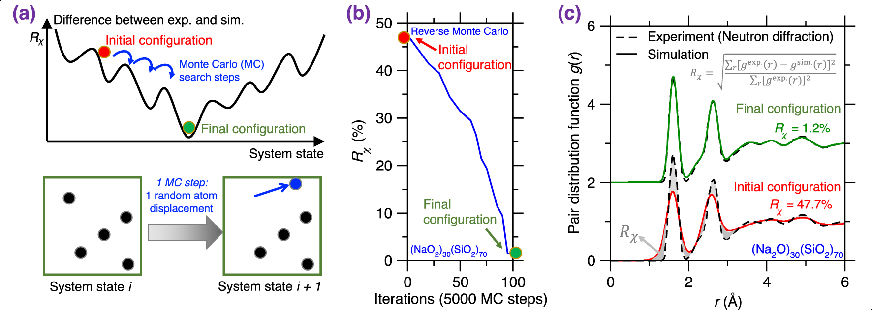

2.2.3. Structural match to experimental data

RMC simulations generally yield atomistic structures that exhibit an excellent agreement with the experimental data that are used to define the cost function (e.g., PDF) [Keen and McGreevy 1990], which is not surprising since RMC solely aims to minimize the difference between simulated and experimental structural data. Figure 3b shows the evolution of the cost function R_𝜒 as a function of the number of MC search steps during the RMC simulation of a sodium silicate glass ((Na₂O)₃₀(SiO₂)₇₀) [Zhou et al. 2020], wherein the cost function is defined based on the neutron PDF. As expected, R_𝜒 gradually decreases and, finally, the simulation generates an atomistic structure that exhibits an excellent match with experimental data. Further, Figure 3c shows the PDF g(r) computed both at the start and end of the RMC simulation. As expected, the final configuration exhibits an excellent agreement with the experimental reference, i.e., the measured g(r) [McGreevy 2001; Pandey et al. 2015; Zhou et al. 2020].

RMC simulations have successfully been used to reveal the structure of a variety of glasses or amorphous solids, especially in the case of systems that are too complex to be simulated by MD or for which no reliable empirical forcefield is available. Example of simulated systems include nuclear waste glasses [Bouty et al. 2014], metal-organic frameworks (MOFs) [Beake et al. 2013; Gaillac et al. 2017], calcium carbonate [Fernandez-Martinez et al. 2013; Goodwin et al. 2010], etc. Overall, RMC simulations offer a powerful tool to model glasses when accurate experimental data are available [Playford et al. 2014].

Figure 4.
(a) Numerical algorithm of molecular dynamics (MD) simulation, which consists of an iterative succession of four computational steps (see text for details) [Takada 2021]. Ab initio MD computes the potential energy U({r_i}) based on first-principles electronic interactions [Boero et al. 2015], whereas, in classical MD, the interatomic interaction is approximately estimated by some empirical functionals [Huang and Kieffer 2015]. (b) Schematic illustrating a melt-quenching simulation for glassy silica. After an initial SiO₂ configuration is prepared, the system is melted under high temperature in the NVT ensemble (or other ensembles, e.g., NPT ensemble), quenched with a given cooling rate to a low temperature, and finally relaxed at this temperature [Carré et al. 2016]. From the viewpoint of the potential energy landscape (PEL) [Wilkinson and Mauro 2021], starting from the high-energy, ergodic liquid state, the system gradually evolves to some nonergodic, low-energy states and finally gets trapped in a local minimum corresponding to a glassy state [Debenedetti and Stillinger 2001; Goldstein 1969].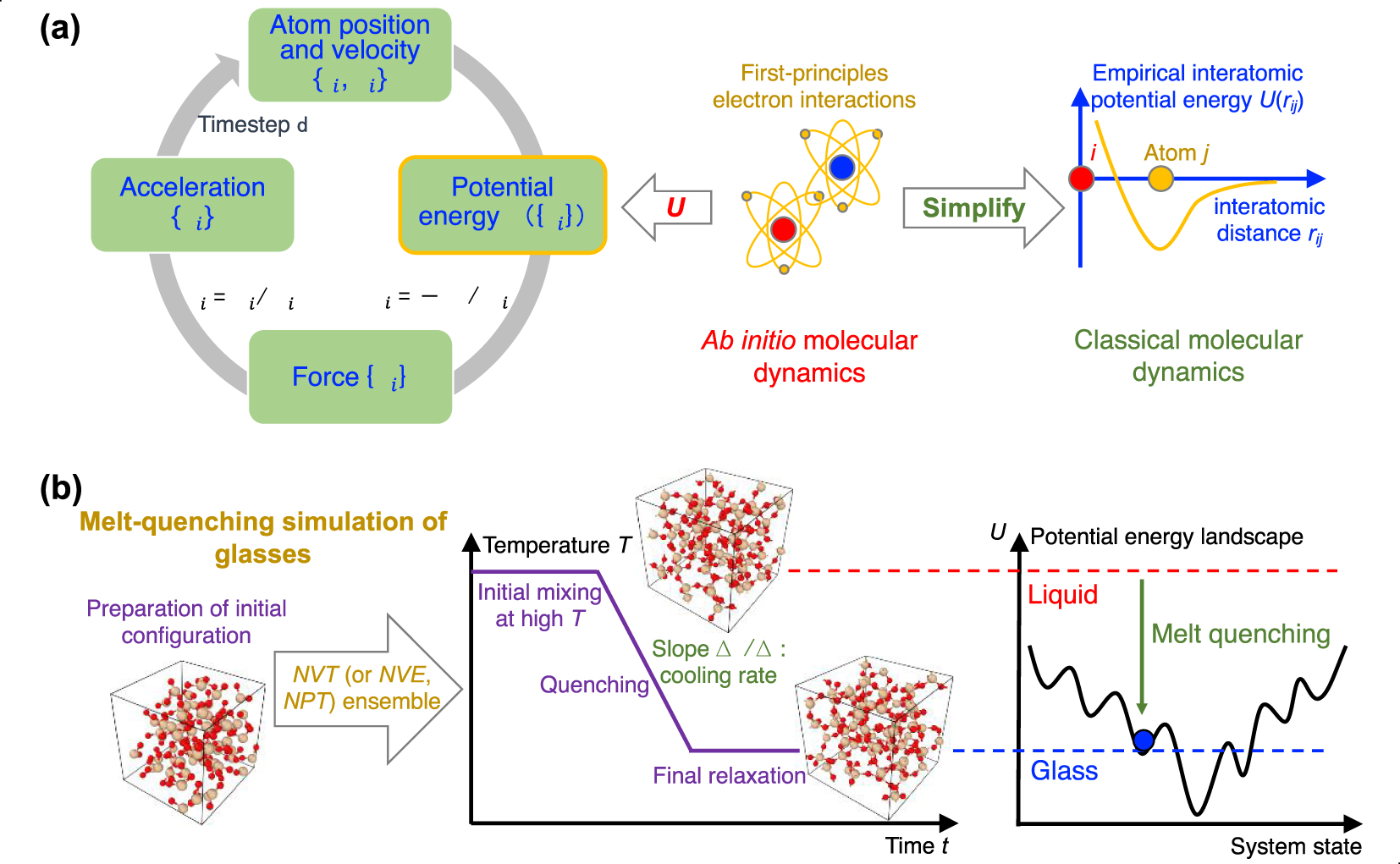

2.3. Molecular dynamics (MD) simulations

MD simulations rely on interatomic forcefields to predict the trajectory of the atoms according to Newton’s law of motion [Alder and Wainwright 1960, 1959; Rahman and Stillinger 1971; Stillinger and Rahman 1974]. Despite their short timescale [Li et al. 2017], MD simulations reproduce the formation process of glasses (e.g., melt quenching process under high cooling rate) to form the atomistic structure of a glass [Bauchy 2014; Micoulaut et al. 2013]. In this section, we provide some general guidelines to implement MD simulations of glasses.

2.3.1. Numerical algorithm

The algorithm of MD simulations consists of a loop of four successive steps (see Figure 4a) [Allen and Tildesley 2017; Takada 2021], namely, (i) computing the system’s potential energy U({r_i}) by summing up all interatomic interactions for the current atom positions {r_i}, (ii) calculating the resultant force {F_i} experienced by each atom i via energy differentiation (i.e., F_i = −∂U∕∂r_i), (iii) obtaining each atom’s acceleration {a_i} from {F_i} as per Newton’s law of motion, that is, a_i = F_i∕m_i, where m_i is the mass of atom i, and finally, (iv) updating the atom positions and velocities after a small, fixed timestep via numerical integration (e.g., Verlet or leapfrog algorithm) [Allen and Tildesley 2017]. Eventually, this four-step loop yields the position of the atom as a function of time, that is, the trajectory of each atom.

It should be pointed out that the accuracy of an MD simulation depends on (i) the realistic nature of the initial configuration (i.e., initial positions and velocities), (ii) the value of the integration timestep, and, importantly, (iii) the accuracy of the interatomic potential energy. First, in the case of the glasses, the initial configuration is usually constructed by randomly placing some atoms in a cubic box while ensuring the absence of any unrealistic overlap (see below). The configuration is then relaxed at elevated temperature until the system loses the memory of its initial configuration. At this point, the outcome of the simulation does not depend any longer on how realistic the initial configuration was. Second, the integration timestep needs to be small enough (∼1 fs) to ensure the accuracy of the numerical integration. In practice, one can check that the timestep is small enough by ensuring the conservation of the system’s total energy and linear/angular momentum during a simulated dynamics in the microcanonical (NVE) ensemble [Grubmüller et al. 1991; Levesque and Verlet 1993; Omelyan et al. 2002]). Third, if the integration timestep is small enough, the accuracy of the MD simulation primarily depends on that of the underlying potential energy (see Figure 4a) [Du 2015; Huang and Kieffer 2015].

Relying on the most fundamental quantum mechanics describing electron interactions (i.e., first-principles calculation of electron interactions) [Hohenberg and Kohn 1964; Kohn and Sham 1965], the interatomic interactions can be accurately computed by conducting first-principles MD simulation (i.e., ab initio MD simulation [Boero et al. 2015], see Section 2.4). Such simulations are computationally expensive but can be used to validate or inform classical MD simulations relying on simplified, empirical potential energy functionals (see Section 2.5) [Carré et al. 2008].

2.3.2. Thermodynamical ensembles

A direct numerical solution of Newton’s law of motion yields the microcanonical NVE dynamics of the N atoms, that is, wherein the total energy and volume of the system are conserved. However, the NVE ensemble does not always mimic experimental conditions. In practice, a system can either be isolated from the rest of the universe (i.e., presenting a constant energy) or be in contact with a thermostat (wherein the thermostat can provide or receive energy so as to fix the temperature T of the system). The volume V of the system can also either be fixed or variable based on the pressure P imposed by a barostat. As such, the most common thermodynamic ensembles used in MD simulations are the microcanonical (NVE), canonical (NVT), and isothermal–isobaric (NPT) ensembles [Du 2019; Leach 2001]. Simulating the motion of the atoms in a non-NVE ensemble (e.g., NVT or NPT) requires slight modification to the constitutive equations used to calculate the acceleration of each atom [Allen and Tildesley 2017; Du 2019]. On the one hand, simulating a constant-temperature dynamics requires the use of a thermostat-based MD algorithm (e.g., Nosé–Hoover thermostat [Hoover 1985; Nosé 1984,?]) to adjust on-the-fly the atomic velocities so as to achieve a target temperature [Andersen 1980; Martyna et al. 1996]. On the other hand, simulating a constant-pressure dynamics involves the use of a barostat-based MD algorithm [Allen and Tildesley 2017; Leach 2001] (e.g., Nose–Hoover barostat [Martyna et al. 1992]) to adjust on-the-fly the system’s volume so as to achieve a target pressure (or state of stress) [Martyna et al. 1996; Tuckerman et al. 2006]. More details can be found in Allen and Tildesley [2017], Leach [2001].

2.3.3. Melt-quenching simulations

The most common method used in MD to prepare a glass consists in mimicking the experimental melt-quenching process [Soules 1990]. The melt-quenching process is detailed in the following and illustrated by Figure 4b for the case of a silica glass [Carré et al. 2008; Liu et al. 2019e].

First, an initial configuration must be created. To this end, one option is to start with a crystalline configuration (e.g., α-quartz in the case of a silica glass). However, this is often not the preferred option as (i) there might not exist a crystal with the same composition as that of the target glass, (ii) the crystal might have a very different density from that of the glass, (iii) the shape of the unit cell of the crystal (e.g., triclinic unit cell) might result in an unnecessarily complicated simulation box geometry, and (iv) melting the initial crystalline structure might require high temperature and/or long simulation time. As an alternative—often preferred—option, the initial configuration can be prepared by randomly placing atoms or molecules (e.g., SiO₂ molecules in the case of a silica glass) into a cubic simulation box with periodic boundary conditions (PBC) [Leach 2001]. The box size can either be fixed so as to match the experimental density of the glass (if when the quenching is performed in the NVT ensemble) or to an arbitrary value (if the quenching is performed in the NPT ensemble). Note that, when creating the initial configuration, care must be taken to avoid any unrealistic atom overlap that might cause spurious fast atom motions at the beginning of the simulation [Martínez et al. 2009]. This can be achieved by imposing a cutoff threshold when randomly placing the atoms, e.g., by ensuring that the distance between a pair of atoms is never lower than the sum of their radii or that a pair of cations (or anions) are never close to each other.

Second, the initial configuration must be melted at high temperature so as to fully lose the memory of the initial configuration. The choice of the melting temperature depends on the type of glass that is considered. On the one hand, the temperature must be high enough to ensure that the atoms move fast enough to “reset” the initial configuration or fully melt the initial crystal. On the other hand, a temperature that is too high might induce some spurious instabilities (e.g., due to the “Buckingham catastrophe” [Carré et al. 2008] or if the system approaches the vaporization point) and increase the length of the simulation (since, at fixed cooling rate, a higher initial temperature increases the duration of cooling). The fact that the initial melting is long enough to ensure that the system has lost the memory of its initial configuration can be checked by computing the intermediate scattering function (ISF) or, as an approximate rule of thumb, by ensuring that the atoms have, on average, diffused by at least half of the simulation box.

Third, the melt is quenched to the glassy state by decreasing temperature. This is typically achieved by linearly decreasing temperature over time, while other more complicated thermal routes can be considered (e.g., nonconstant cooling rate or step-by-step cooling). The cooling process can either be performed in the NVT or NPT ensemble. The NPT ensemble is usually desirable as it mimics the experimental synthesis of glass (i.e., wherein the melt is quenched under atmospheric pressure). In turn, the NVT ensemble can yield some spurious effects as, since density is fixed, the pressure changes as a function of temperature. As a result, when using the NVT ensemble during cooling, the glass tends to “freeze” under positive (compressive) pressure at the glass transition temperature, which can impact the resulting structure. However, some interatomic forcefields are unable to yield the correct final glass density, so that using the NVT ensemble and fixing the volume to achieve the experimental glass density might, in some cases, be necessary. Due to the high computing cost of MD, the cooling rate (typically 10¹⁴–10⁹ K/s) is much faster than those achieved in conventional experiments (10²–10⁰ K/s) [Li et al. 2017]. From the viewpoint of PEL [Goldstein 1969; Wilkinson and Mauro 2021], the system starts, upon cooling, from a high-energy, ergodic liquid state and gradually evolves to some nonergodic, lower-energy state, before eventually getting trapped in a local minimum corresponding to a glassy state (see Figure 4b) [Debenedetti and Stillinger 2001]. At the end of the cooling process, it is also common to perform an additional relaxation run to ensure that the system has reached a plateau in energy, and volume or pressure (in the NPT and NVT ensembles, respectively).

Fourth, once formed, the glass can be investigated or subjected to additional simulations [Du 2019; Pedone 2009]. Typical investigations include various structural analysis (e.g., coordination number) [Bauchy 2014, 2012], mechanical properties (e.g., strain–stress curve) [Liu et al. 2019b; Yang et al. 2019], thermodynamics (e.g., potential energy) [Bauchy and Micoulaut 2015], and vibrational/dynamical properties (e.g., atom diffusivity) [Bauchy et al. 2013; Bauchy and Micoulaut 2011]. More details can be found in Levchenko et al. [2020], Massobrio [2015]. Note that any statistical analysis must be averaged over a trajectory that is long enough to filter out the effect of statistical fluctuations (the magnitude thereof depending on the size of the simulated system). It is also worth noting that, upon quenching, the glass may end up in notably different regions of the energy landscape [Allen and Tildesley 2017]. As such, it is a good practice to simulate a series of independent melt-quenching simulations for each glass (typically around 3 to 6) and to average results over these simulations.

2.4. Ab initio molecular dynamics simulations

2.4.1. First-principles calculation of interatomic interactions

Figure 5.
(a) Schematic illustrating the basic idea of ab initio molecular dynamics (MD) based on first-principles calculation of the system’s potential energy U (see text for details) [Boero et al. 2015]. (b) Comparison between the pair distribution function (PDF) g(r) computed by neutron diffraction experiment and ab initio MD simulation using the Car–Parrinello (CP) method and generalized gradient approximation (GGA) potential for a GeSe₂ glass [Micoulaut et al. 2013]. The inset is a snapshot of the simulated GeSe₂ glass.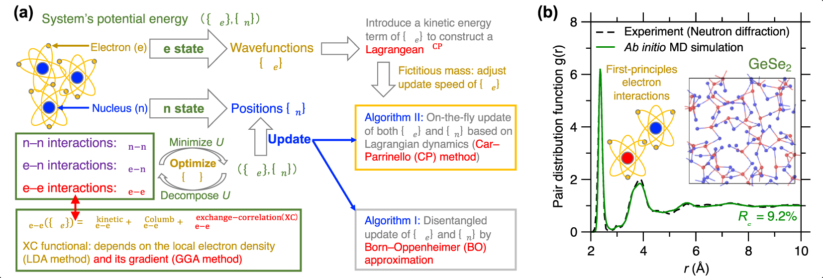

Ab initio MD simulations estimate the interatomic interactions based on first-principles calculation of electron interactions within the framework of density function theory (DFT) [Kohn and Sham 1965; Marx and Hutter 2009; Parr 1980]. Figure 5a illustrates the basic idea of ab initio MD, wherein a glass system’s potential energy U is computed as a function of both the electron wave functions {𝛹_e} (i.e., the electron state) and the nuclei positions {r_n} (i.e., the nuclei state) [Hohenberg and Kohn 1964; Kohn and Sham 1965]. The potential energy U is calculated by summing up three types of interactions in the system [Boero et al. 2015; Marx and Hutter 2009]:

\begin{matrix} U ({𝛹_{e}}, {r_{n}}) & = & U_{n - n} ({r_{n}}) + U_{e - n} ({𝛹_{e}}, {r_{n}}) \\ + U_{e - e} ({𝛹_{e}}) \end{matrix}

(3)

where the right-hand terms refer to nucleus–nucleus interactions U_n–n, electron–nucleus interactions U_e–n, and electron–electron interactions U_e–e, respectively. U_e–n can be estimated using the pseudopotential (PP) approach [Hamann et al. 1979; Troullier and Martins 1991; Vanderbilt 1990] wherein core electrons (close to the nucleus, where the electron–nucleus interaction varies rapidly in space) are filtered out as they do not engage in the creation of chemical bonding. Rather, interatomic interactions arise from valence electrons (far away from the nucleus) that form chemical bonds [Bachelet et al. 1982]. The PP approach then fits a potential describing the interaction between nucleus and valence electrons, where the fitting uses as reference the all-electron state solution of the ground-state single atom model [Hamann et al. 1979]. Based on the PP approach [Troullier and Martins 1991], U_n–n is simply the Coulombic interaction between nuclei presenting their net valence charge [Boero et al. 2015].

2.4.2. Choice of exchange-correlation (XC) potential

U_e−e is a key ingredient in first-principles simulation. It can be further described by three types of energy terms [Boero et al. 2015; Kohn and Sham 1965]:

U_{e - e} ({𝛹_{e}}) = U_{e - e}^{kinetic} + U_{e - e}^{Coulomb} + U_{e - e}^{XC}

(4)

where the right-hand terms represent the electrons’ kinetic energy U^kinetic, Coulombic interaction U^Coulomb, and the exchange-correlation (XC) interaction U^XC, respectively. Note that, the XC interaction is very challenging to describe accurately [Gunnarsson and Jones 1985; Johnson et al. 1993; Perdew and Zunger 1981], as it depends not only on the local electron density but also on its spatial gradient [Langreth and Mehl 1983; Perdew et al. 1996a]. Assuming that the local electron density is homogeneous, the local density approximation (LDA) method can be used to estimate U^XC [Fulde 1995; Kohn and Sham 1965], which has been proved to offer satisfactory descriptions of XC interactions [Cobb et al. 1996]. However, it should be pointed out that, in many cases (e.g., glasses exhibiting structural heterogeneities [Micoulaut et al. 2013]), assuming a homogeneous local electron density results in an inaccurate estimation of U^XC [Langreth and Mehl 1983; Micoulaut et al. 2009]. To address this issue, some generalized gradient approximation (GGA) methods have been developed to construct more accurate XC functionals with respect to the electron density gradient [Perdew et al. 1996a, b]. More details can be found in Fulde [1995], Marx and Hutter [2009].

2.4.3. Numerical algorithms

Based on all these formulations of first-principles interatomic interactions [Boero et al. 2015; Marx and Hutter 2009], the system’s ground-state potential energy U({𝛹_e},{r_n}) can be calculated via optimizing {𝛹_e} so as to minimize U for the current nuclei positions {r_n} (see Figure 5a) [Hafner 2008; Pople et al. 1989]. After updating the new nuclei positions {r_n} after a small timestep, the system’s potential energy U is then recomputed through optimizing {𝛹_e} [Boero et al. 2015]. Two algorithms have been developed to optimize {𝛹_e} and update {r_n} [Niklasson et al. 2006], viz., (i) the Born–Oppenheimer (BO) approximation to disentangle the updates of {𝛹_e} and {r_n} [Boero et al. 2015; Niklasson et al. 2006], wherein {𝛹_e} is recomputed at each timestep and offers an accurate estimation of the potential energy U to update the nuclei positions {r_n}, and (ii) the Car–Parrinello (CP) method to construct a Lagrangian L^CP({𝛹_e},{r_n}) that updates both quantities on-the-fly based on Lagrangian dynamics [Car and Parrinello 1985], where L^CP includes a constructed kinetic energy term of {𝛹_e} by assigning to {𝛹_e} a fictitious electronic mass that dictates the update inertia of {𝛹_e} [Boero et al. 2015]. In practice, systems with slow change of nuclei positions tend to require a large fictitious mass to delay the update of {𝛹_e} as well as a large timestep to accelerate the update of {r_n} [Car and Parrinello 1985]. In other words, when running a CP-MD simulation, one needs to select a proper set of timestep and fictitious mass large enough to (i) reduce the computation cost of the update of {𝛹_e} and {r_n} but also small enough to (ii) numerically conserve the system’s energy and linear/angular momentum [Boero et al. 2015]. More details can be found in Boero et al. [2015], Marx and Hutter [2009].

2.4.4. Applications and limitations

Since ab initio MD simulations are typically able to accurately describe interatomic interactions [Pople et al. 1989], they are the method of choice to simulate complex glasses for which no robust empirical forcefields are available (see below). This is typically the case for glasses exhibiting complex bonds (i.e., with a mixed ionic/covalent/metallic character or varying electronic delocalization) or flexible local structures (e.g., varying coordination numbers) [Massobrio 2015]. For example, chalcogenide glasses (e.g., Ge–Se glasses) typically exhibit complex structural features that cannot be accurately reproduced by classical MD [Mauro and Varshneya 2006], including under- and over-coordinated atoms, edge-sharing structures, and homopolar bonds (see insert of Figure 5b) [Petri et al. 2000]. Figure 5b shows a melt-quenched GeSe₂ glass prepared by ab initio MD simulation, wherein its computed PDF g(r) is compared with neutron diffraction data [Micoulaut et al. 2013]. Relying on CP-MD method and GGA-XC potential [Car and Parrinello 1985; Perdew et al. 1996a], the simulation offers a glass structure that is in excellent agreement with experimental data [Micoulaut et al. 2009].

However, despite their unparalleled predictive power [Pople et al. 1989], ab initio simulations still come with a series of limitations. First, although they rely on a fundamental description of electronic interactions, they still rely on a number of assumptions (e.g., choice of the pseudopotential and exchange-correlation function). Second, ab initio MD simulations come with a computational cost that is orders of magnitude larger than that of classical MD [Marx and Hutter 2009]. This limits the timescale that is accessible to ab initio MD simulations (typically to 100s of ps) [Boero et al. 2015]. This restricts their use to high cooling rates, which, in turn, tends to yield glasses that are more disordered (higher fictive temperature) than their experimental counterparts [Li et al. 2017]. Finally, the computational cost of ab initio MD simulations typically scales with the cube of the number of electronic degrees of freedom [Hafner 2008]. As a result, ab initio MD simulations are usually limited to very small systems (up to a few hundred atoms) [Massobrio 2015]. This prevents their use in capturing small compositional effects (since replacing one atom by another largely affects the overall composition in a small system) or extended structural features (e.g., large rings or compositional heterogeneity) [Du and Corrales 2006; Nakano et al. 1994].

Figure 6.
(a) Pair distribution function (PDF) g(r) of a melt-quenched (Na₂O)₃₀(SiO₂)₇₀ glass prepared by a classical MD simulation using an empirical forcefield (here, a Buckingham potential [Cormack et al. 2002], see (5)) and a cooling rate of 0.001 K/ps [Zhou et al. 2020]. The neutron diffraction data is added as a comparison [Wright et al. 1991]. The inset illustrates the shape of this empirical forcefield, i.e., the interatomic potential energy U(r_ij) as a function of interatomic distance r_ij [van Beest et al. 1990]. (b) Schematic illustrating the parameterization of an empirical forcefield by searching for the minimum position (i.e., the optimal forcefield) in a cost function landscape as a function of forcefield parameters [Carré et al. 2016]. The cost function is defined herein as the difference between classical MD result and its ab initio reference [Liu et al. 2019e]. The optimal forcefield is parameterized so as to match ab initio MD simulation and also offers a good agreement with experiment (see panel (a)) [Carré et al. 2008]. Note that several competitive minima (yielding competitive optimal forcefields) can coexist in the cost function landscape (see panel (c)) [Liu et al. 2020a]. (c) Comparison between the PDFs computed by ab initio MD simulation and classical MD simulation using two distinct Buckingham forcefields (with different parameterizations) for a silica liquid. The two potentials are referred to as “soft” (exhibiting weak columbic interactions) and “hard” (exhibiting more intense columbic interactions) [Liu et al. 2020a].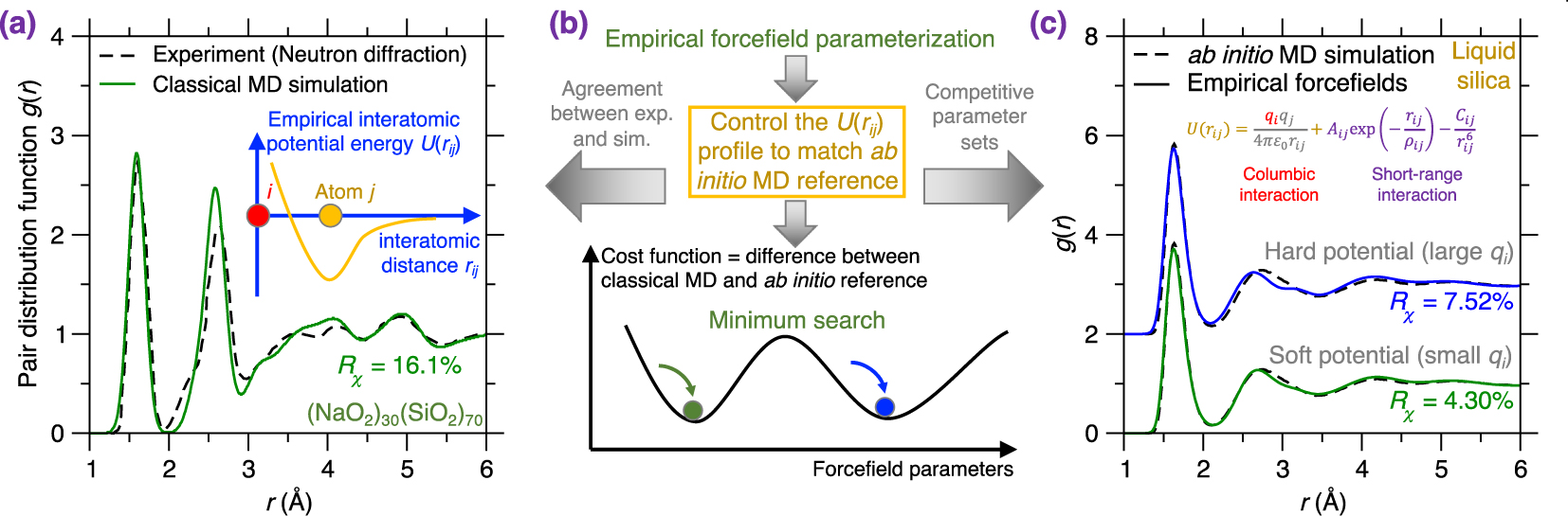

Thanks to their accuracy, ab initio MD simulations have been applied to predict the structure and dynamics of various types of glasses or amorphous solids, including amorphous silicon [Car and Parrinello 1988], chalcogenide [Micoulaut et al. 2013], Ge–Sb–Te phase-change materials [Caravati et al. 2009], MOFs [Darby et al. 2020; Sillar et al. 2009], silicates [Baral et al. 2017; Tilocca and de Leeuw 2006], borates [Scherer et al. 2019], etc. Notably, by accurately describing the interatomic interactions, ab initio MD offers a powerful tool to simulate complex glasses that cannot be properly described by empirical forcefields.

2.5. Classical molecular dynamics simulations

2.5.1. Empirical forcefields

In contrast to the explicit description of electronic effects offered by ab initio MD [Marx and Hutter 2009], classical MD relies on empirical forcefields to describe interatomic interactions—via physics/intuition-based, computationally efficient functionals [Massobrio 2015]. For example, Figure 6a shows the PDF g(r) of a melt-quenched (Na₂O)₃₀(SiO₂)₇₀ glass prepared by classical MD simulation using an empirical forcefield [Cormack et al. 2002; Du and Cormack 2004]. The neutron diffraction data is added as a reference for comparison [Wright et al. 1991]. Notably, this empirical forcefield offers an atomistic structure that is in good agreement with experimental data. Note that the simulated and experimental glasses are prepared with different cooling rate [Li et al. 2017]. The good agreement between simulated and experimental PDFs (see Figure 6a) suggests that, although the empirical forcefield is a simplification of the real interatomic interactions [Huang and Kieffer 2015; van Beest et al. 1990], it can accurately describe them while relying on a significantly reduced computational cost as compared to first-principles calculations [Bauchy et al. 2013; Carré et al. 2008]. Thanks to its much faster execution time as compared to ab initio MD simulation, classical MD simulation can extend to much longer timescales (up to a few nanoseconds) and larger length scales (up to millions of atoms) [Lane 2015; Plimpton 1995a].

2.5.2. Forcefield functionals

The optimal functional form of the empirical interatomic potential depends on the type of glass that is simulated (e.g., ionic, covalent, metallic glass, etc.) and no “universal” empirical potential is available to date [Du 2015; Huang and Kieffer 2015].

In practice, ionocovalent glasses (e.g., silicate glasses, which feature ionocovalent bonds [Huang and Kieffer 2015]) can be well described by a combination of: (i) long-range coulombic interactions and (ii) a Buckingham-format functional description of short-range interactions to compute the potential energy U(r_ij) between atom i and atom j at a distance r_ij (see inset of Figure 6a) [Carré et al. 2008; Du and Corrales 2006; van Beest et al. 1990]:

U (r_{ij}) = \frac{q_{i} q_{j}}{4 π 𝜀_{0} r_{ij}} + A_{ij} exp (- \frac{r_{ij}}{𝜌_{ij}}) - \frac{C_{ij}}{r_{ij}^{6}}

(5)

where q_i is the partial charge of atom i, 𝜀₀ is the dielectric constant, and A_ij, 𝜌_ij, and C_ij are parameters describing short-range interactions [Du and Corrales 2006]. These parameters are adjusted for each pair of elements (e.g., Si–O) so as to achieve a good agreement with experimental or ab initio references (see below) [Sundararaman et al. 2018; van Beest et al. 1990]. In particular, the well-established Teter potential [Cormack et al. 2002] has been demonstrated to offer an accurate description of various structural, thermodynamical, and dynamical properties of silicate glasses [Bauchy 2012; Bauchy et al. 2013; Du and Cormack 2004; Du and Corrales 2006].

Note that, in the case of interactions that rapidly converge to zero upon increasing distance (e.g., Van der Waals interactions, which is proportional to 1/r⁶), the energy error associated with the fact of using a finite cutoff converges to zero as the cutoff increases. However, this is not the case for Coulombic interactions, which exhibit a slow decrease upon increasing distance r (i.e., proportional to 1/r). In such a case, the energy contribution that is neglected when using a cutoff (arising from long-distance interactions between atoms) does not converge to zero upon increasing cutoff. As such, long-range Coulombic interactions (including across PBC) must be explicitly considered to ensure the accuracy of the simulation. In practice, computing Coulombic interactions is often the most computationally expensive step when simulating ionocovalent glasses. In that regard, various summation methods have been developed to speed up the computation of electrostatic interactions, such as the Ewald method [Ewald 1921], particle–particle–particle–mesh (PPPM) method [Hockney and Eastwood 1988], and damped-shifted-force (DSF) method [Fennell and Gezelter 2006]. In detail, both the Ewald and PPPM methods are based on the idea that the summation of long-range interactions can be efficiently calculated in the reciprocal space using a Fourier transform [Allen and Tildesley 2017]. Unlike the Ewald or PPPM methods, the DSF method is conducted in real space and is based on the rapidly converging summation of a short-range potential—whose cutoff is large enough—to approach the effective long-range Coulombic interactions [Fennell and Gezelter 2006]. In practice, both the Ewald and PPPM summation methods offer accurate calculations of the Coulombic interactions. In many cases, electrostatic interactions can also be reasonably well approximated by the DSF method [Carré et al. 2007; Fennell and Gezelter 2006], which, in turn, is significantly more computationally efficient than Ewald and PPPM since it does not involve any Fourier transform [Fennell and Gezelter 2006].

It is worth pointing out that, as the accuracy of classical MD simulations significantly relies on the analytical formulation of the empirical forcefield, it is necessary, when developing empirical forcefield functionals, to account for all essential components of the interaction (e.g., Coulombic component of ionocovalent interaction) that affect the targeted glass properties. Indeed, although select properties are not very sensitive to the details of a forcefield (e.g., density or PDF), other properties can be strongly affected by small variations in the parameters or analytical formulation of the empirical potential. In such cases, it may be necessary to develop advanced forcefields that are able to capture some complex chemical or physical behaviors, including bond formation/breaking, charge transfers, polarization effects, short-range repulsion, etc. [Jahn et al. 2006; Jahn and Madden 2007; Serva et al. 2020]. In that regard, some advanced forcefields such as the aspherical ion model (AIM)—which is more complex than the Buckingham potential [Liu et al. 2020a]—have been developed to account for these essential, complex interaction behaviors in studying the dynamics of complex oxides [Jahn et al. 2006; Jahn and Madden 2007; Serva et al. 2020]. Note that, although such potentials are more computationally expensive, they generally show an improved level of agreement with experiments and a high transferability upon composition, temperature, and pressure changes [Jahn et al. 2006; Jahn and Madden 2007; Serva et al. 2020].

In contrast to ionocovalent glasses, covalent glasses (e.g., amorphous silicon [Stillinger and Weber 1985] or chalcogenide glasses [Micoulaut et al. 2013]) cannot be described by 2-body interatomic potentials due to the directional nature of the covalent bonds they form [Phillips 1981, 1979]. As such, describing covalent glasses requires the use of 3-body potential interactions—e.g., Stillinger–Weber (SW) potential [Ding and Andersen 1986; Stillinger and Weber 1985]—to constraint the values of the interatomic angular interactions between a central atom i and its two neighbor atoms j and k [Du 2015; Mauro and Varshneya 2006]:

\begin{matrix} U (r_{ij}, r_{ik}, 𝜃_{ijk}) & = & \sum_{i} \sum_{j > i} 𝜙_{2} (r_{ij}) \\ + \sum_{i} \sum_{j \neq i} \sum_{k > j} 𝜙_{3} (r_{ij}, r_{ik}, 𝜃_{ijk}) \end{matrix}

(6)

where 𝜙₂ and 𝜙₃ represent, respectively, the radial 2-body interaction and angular 3-body interaction term, as a function of the interatomic distance r_ij, r_ik, and the bond angle 𝜃_ijk between the vectors r_ij and r_ik. More details can be found in Du [2019], Mauro and Varshneya [2006], Stillinger and Weber [1985].

Finally, the simulation of metallic glasses typically requires the description of many-body effects [Pelletier and Qiao 2019; Sheng et al. 2006], which can be well described by the Embedded Atom Method (EAM) potential [Daw et al. 1993]. In the EAM approach, the potential energy U_i of a central atom i is formulated as [Daw and Baskes 1984, 1983]:

U_{i} = f_{𝛼} (\sum_{j \neq i} 𝜌 𝛽 (r_{ij})) + \frac{1}{2} \sum_{j \neq i} 𝜙_{𝛼 𝛽} (r_{ij})

(7)

where F is the energy gained by embedding the cation i in the “ocean” of delocalized electrons described by the local atomic electron density 𝜌, 𝜙 is a pair potential interaction describing the cation–cation interactions, 𝛼, 𝛽 represent element type of atom i and j, respectively, and j denotes the neighbors of atom i within a radius cutoff r_c. More details can be found in Daw et al. [1993], Daw and Baskes [1983].

Note that, to reduce the computational cost associated with the calculation of the empirical forcefields, a cutoff r_c is typically adopted—wherein the interaction energy between a pair of atoms is assumed to be zero if their distance exceeds the cutoff [Chialvo and Debenedetti 1990; Du 2015]. In addition, a neighbor list algorithm is typically adopted to reduce the number of times the distance between a pair of atoms is calculated [Allen and Tildesley 2017; Leach 2001].

2.5.3. Forcefield parameterization

In addition to the choice of its functional form [Du 2015], the accuracy of an empirical forcefield strongly depends on its parameterization [Sundararaman et al. 2020, 2018; Wang et al. 2018]. Figure 6b illustrates the general idea behind the parameterization of an empirical potential. Such parameterization can be formulated as an optimization problem, wherein the forcefield parameters are optimized so as to minimize a given cost function. This problem can be illustrated in terms of a cost function landscape, which represents the topographical evolution of the cost function as a function of the forcefield parameters. The cost function captures the level of mismatch between a simulated metric and a given reference value. The simulated metric can be the interatomic energy/force, some structural features (e.g., PDF), or some other macroscopic properties (e.g., density, stiffness, etc.).

For each type of metric, reference values can be offered by experimental data or ab initio simulations. On the one hand, defining the cost function in terms of the level of mismatch between computed and experimental data tends to yield a good agreement between simulated and experimental glass properties—since the parameterization scheme specifically aims to minimize this difference. However, on the other hand, it is not always meaningful to compare a simulated glass with its experimental counterpart. Indeed, glasses simulated by MD are prepared with a cooling rate that is significantly higher than those experienced in traditional experiments and, therefore, should be different (typically more disordered) than their experimental counterparts [Carré et al. 2016; Li et al. 2017; Vollmayr et al. 1996b]. Hence, parameterizing an empirical forcefield so as to “force” a simulated glass to exhibit properties that match experimental data may yield an unrealistic forcefield. That is, forcing simulated and experimental glasses to feature similar properties can typically only be achieved by “mutual compensations of errors”, that is, wherein the forcefield is deformed so as to compensate the fact that the simulated glass is prepared with an extremely high cooling rate. As such, although such parameterization may offer an apparent agreement between simulations and experiments for the properties that are included in the cost function, the resulting forcefield, due to its nonphysical nature, may dramatically fail at predicting properties that are not included in its cost function. In contrast, parameterizing a forcefield so as to match with ab initio data is expected to yield a more realistic description of the true interatomic potential. However, glasses prepared with such a realistic forcefield should be compared to hyperquenched glasses (i.e., prepared under high cooling rate) and, hence, may not exhibit a good agreement with experimental data prepared under slower cooling rates.

In terms of the metric to be considered in the cost function, it has recently been suggested that, in the case of glasses or liquids, using a structural property as reference (e.g., PDF) tends to offer better results than directly forcing the parameterized forcefield to match reference force values (as computed by ab initio simulations) [Carré et al. 2016, 2008]. In the example shown in Figure 6c, the cost function R_𝜒 is defined as the magnitude of the difference between the PDF g(r) computed by classical MD and ab initio MD for a liquid silica system [Liu et al. 2019e]. Note that parameterizing this forcefield based on liquid (rather than glassy) configurations effectively removes any spurious effects arising from the thermal history of the system.

Various optimization methods are available to “navigate” the cost function landscape, that is, to identify the optimal forcefield parameters that minimize the cost function [Carré et al. 2016], including MC search [Iype et al. 2013], Bayesian optimization [Liu et al. 2019c, e], particle swarm optimization [Christensen et al. 2021], or gradient descent search [Shewchuk 1994]. Note that this optimization problem is typically ill-defined since several degenerate sets of forcefield parameters can often minimize the cost function, that is, several competitive minimum positions can be found in the cost function landscape [Liu et al. 2020a, 2019c]. Figure 6c illustrates two competitive forcefields based on the same Buckingham-format functional [van Beest et al. 1990] (see (5)). These forcefields can be described as “soft” (featuring weak coulombic interactions) and “hard” (featuring more intense coulombic interactions) and both offer a competitive minimum value of the cost function R_𝜒 for silica liquids [Liu et al. 2020a]. Nevertheless, despite the apparent harmony, the atomistic structures offered by the soft and hard potential exhibit pronounced differences for structural features that are not included in the cost function (e.g., bond angular distribution or ring size distribution) [Liu et al. 2020a]. This exemplifies the need to a posteriori validate forcefields that validate the accuracy of forcefields after their parameterization [Liu et al. 2019c].

Finally, it is worth pointing out that both the choice of forcefield functionals and forcefield parameterization can affect the forcefield’s transferability as a function of, for instance, glass composition, pressure, or temperature [Hernandez et al. 2019; Jahn and Madden 2007]. Indeed, forcefields are often developed for a specific glass composition and range temperature/pressure (e.g., liquid silica). In general, there is no guarantee that such forcefields can offer realistic predictions far from the conditions used during their training [Sundararaman et al. 2020, 2018]. For instance, certain chemical behaviors—e.g., charge transfers—may not be similar under various conditions of temperature or pressure and, hence, may require some adjustments in the parameterization of empirical forces to be properly accounted for [Liu et al. 2020a]. The transferability of forcefields is also likely to be poor when the forcefield is used under conditions wherein the atoms exhibit some local environments (e.g., varying coordination numbers) that are different from those observed during the training of the forcefield. This limitation is especially pronounced for borate glasses (wherein the average coordination number of boron depends on temperature) and pressurized glasses (wherein coordination numbers tend to increase under pressure) [Salmon and Zeidler 2015]. In order to overcome these limitations and develop transferable forcefields, one first needs to propose a forcefield functional that is complex enough to capture the nature of interatomic interactions in all the conditions of interest (e.g., Buckingham-format potential for ionocovalent bond interactions in silicate glasses), but generic enough to avoid any unrealistic extrapolations due to “overfitting” [Du 2015; Huang and Kieffer 2015]. Then, the transferability of a forcefield greatly depends on its forcefield parameterization scheme, where the cost function should be designed so as to consider the structure and properties of glasses under different conditions [Liu et al. 2019c; Sundararaman et al. 2018]. Note that there always exists a balance between (i) the ability of a forcefield to accurately predict the unique, detailed properties of a specific system and (ii) the capability of a forcefield to offer a robust transferability for a wide range of compositions and conditions [Liu et al. 2019c]. To address the issue of transferability, several recent works have focussed on developing generic forcefields that can be applied to a large compositional envelope at the expense of potentially being unable to capture the fine structural details of a specific composition [Hernandez et al. 2019; Jahn and Madden 2007], including the well-established Teter potential for modified silicate glasses [Du and Corrales 2006], the Wang–Bauchy potential for borosilicate glasses [Wang et al. 2018], etc.

Thanks to their high computational efficiency as compared to ab initio simulations [Carré et al. 2008; Huang and Kieffer 2015], classical MD simulations relying on empirical forcefields have been extensively used to model glasses [Cormier et al. 2003; Mead and Mountjoy 2006; Tanguy et al. 1998]. Simulated systems include glassy silica [Carré et al. 2008; Liu et al. 2020a; van Beest et al. 1990], modified (e.g., alkali) silicate glasses [Cormack and Du 2001], aluminosilicate glasses [Bouhadja et al. 2013], borates [Kieu et al. 2011; Sundararaman et al. 2020; Wang et al. 2018], etc. It should be pointed out that, as the number of elements in the glass increases, it becomes extremely challenging to properly describe all the distinct interactions between pair of elements (since the number of parameters that need to be adjusted scales with the square of the number of elements) [Du 2015].

2.6. Reactive molecular dynamics simulations

2.6.1. Gap between ab initio and classical MD simulations

In contrast to classical MD, ab initio MD can accurately describe a chemical reaction process but is limited to small system size (up to hundreds of atoms) [Boero et al. 2015], while, in turn, classical MD can extend to large systems (up to millions of atoms) but lack an accurate description of chemical reaction processes [Plimpton 1995a; Senftle et al. 2016]. Although classical MD simulations exhibit high computation efficiency [Marx and Hutter 2009; Massobrio 2015], they rely on simplified empirical forcefields, which may accurately predict certain properties (e.g., PDF g(r)) of glasses but may not offer robust predictions for more complex properties that are more sensitive to the details of the forcefields [Ganster et al. 2007; Ispas et al. 2002]. In addition, classical MD simulations relying on static forcefields and fixed charges are often unable to robustly account for charge transfer mechanisms and defective coordinated states, which prevents such simulations from properly describing the breaking and formation of bonds during chemical reactions [Buehler et al. 2006; Deng et al. 2021; Du et al. 2019a; Yu et al. 2018]. To address this limitation, reactive MD simulations—i.e., MD relying on reactive forcefields (e.g., ReaxFF) [van Duin et al. 2003, 2001]—have been proposed as an intermediate option, in between classical and ab initio MD. The promise of reactive MD is to offer an accuracy that approaches that of ab initio MD while involving a computational burden that is more comparable to that of classical MD. This makes it possible for reactive MD to simulate fairly large systems (up to tens of thousands of atoms) over extended time scales (up to a few nanoseconds) with an enhanced accuracy as compared to classical MD (see Figure 7a) [Senftle et al. 2016]. However, reactive forcefields typically rely on hundreds-to-thousands of parameters and, hence, are extremely challenging to parameterize. This has thus far limited their applications to a small number of glass families [Senftle et al. 2016].

Figure 7.
(a) Illustration of reactive molecular dynamics (MD) simulations relying on reactive forcefield (e.g., ReaxFF) to bridge the gap between ab initio and classical MD, both in terms of range of system size and accuracy [Senftle et al. 2016]. (b) Illustration of the sol–gel formation process of glassy silica in terms of the potential energy landscape (PEL) predicted by ab initio MD, reactive MD, and classical MD [Du et al. 2018; Steinfeld et al. 1999]. Using the ab initio PEL as a reference, reactive MD shows a more accurate transition energy than classical MD [Du et al. 2018], on account of the fact that the ReaxFF forcefield explicitly models dynamical bond formations and charge transfers during the chemical reaction [van Duin et al. 2003]. (c) Comparison between the neutron structure factor S_N(Q) computed by classical MD and reactive MD for a sodium silicate glass ((Na₂O)₃₀(SiO₂)₇₀) [Yu et al. 2017a]. The same experimental S_N(Q) is added as a reference [Grimley et al. 1990].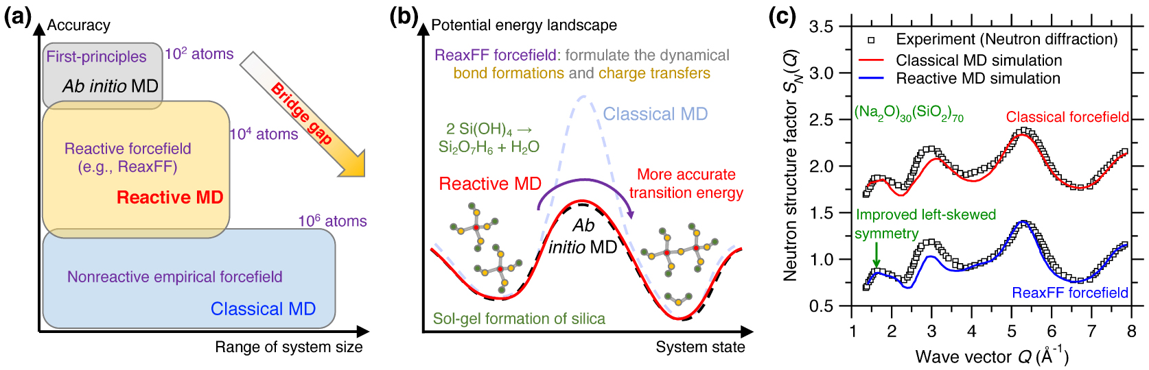

2.6.2. ReaxFF forcefield

The ReaxFF forcefield is one of the most popular implementations of reactive MD [Leven et al. 2021]. As detailed in the following, the key advantages of ReaxFF are that it (i) explicitly describes the dynamical formations and breaking of bonds, (ii) accounts for charge transfers between atoms, and (iii) dynamically adjusts the interatomic interactions as a function of the local environment of each atom [van Duin et al. 2003, 2001]. This makes it possible to describe phase transitions, defect formations, or chemical reactions between atoms (e.g., to simulate the reactivity of a glass surface with water) [Buehler et al. 2006; Du et al. 2018].

In detail, the ReaxFF forcefield calculates the system’s potential energy U_sys by summing up the following energy terms [van Duin et al. 2003]:

\begin{matrix} U_{sys} & = & U_{bond} + U_{vdWaals} + U_{Coulomb} + U_{under} + U_{over} \\ + U_{lp} + U_{val} + U_{tors} + U_{conj} + U_{pen} \end{matrix}

(8)

where the right-hand terms refer, respectively, to the short-range bond energy, Van der Waals energy, Coulomb potential energy, under-coordination energy, over-coordination energy, long-range electron pairs energy, valence angle energy, torsion energy, conjugation energy, and penalty energy. A detailed description of these terms can be found in Senftle et al. [2016], van Duin et al. [2003, 2001]. Importantly, ReaxFF is a bond-order-based forcefield, that is, the energy terms are generally formulated as a function of the local bond order of each atom, which is dynamically determined by its local environment [van Duin et al. 2003]. This bond-order formulation enables reactive MD to capture the dynamical process of bond formations and dissociations. Moreover, in contrast to classical MD simulations relying on fixed charges [Liu et al. 2019e; van Beest et al. 1990], the charges of the atoms are dynamically assigned based on a charge equilibration (QEq) method [Rappe and Goddard 1991], which captures the occurrence of charge transfers during bond breakages and reformations. All these features—i.e., dynamical bond formations and charge transfers—render ReaxFF ideal to simulate chemical reactions [Senftle et al. 2016].

2.6.3. Glass reactivity

Reactive MD simulations offer an ideal tool to investigate the chemical reactivity of glasses [Senftle et al. 2016]. For instance, Figure 7b illustrates the sol–gel formation process of glassy silica (in terms of the condensation of Si(OH)₄ precursors) from the viewpoint of an energy state transition in PEL [Du et al. 2018; Steinfeld et al. 1999]. Classical MD relying on empirical forcefield (e.g., Buckingham potential [van Beest et al. 1990]) generally offers an accurate description of near-equilibrium properties (i.e., around local minimum energy states) but typically fails at properly describing far-from-equilibrium behaviors like those experienced in transition states [Liu et al. 2019e]. In particular, classical MD typically does not offer realistic energy barrier predictions [Du et al. 2018]. In contrast, reactive MD (e.g., based on ReaxFF) can offer more accurate description of transition energy barriers, which makes it possible to simulate sol-to-gel transitions [Du et al. 2019b, 2018; Zhao et al. 2021, 2020]. Reactive potentials also make it possible to model the reactivity of glass with aqueous solutions [Deng et al. 2019; Du et al. 2019a; Fogarty et al. 2010; Mahadevan and Du 2020; Yu et al. 2018]. The description of bond formation/breaking also make reactive MD simulations an ideal tool to study fracture processes [Bauchy et al. 2016, 2015; To et al. 2020] or vapor deposition processes [Wang et al. 2020].

2.6.4. Glass structure

The fact that ReaxFF can dynamically adjust interatomic interactions as a function of the local environment of each atom is also a key advantage in glass simulations—since glasses can exhibit a large variety of local structures (e.g., varying coordination states). As such, when properly parameterized, reactive forcefields have the potential to offer an improved description of the atomic structure of glasses as compared to classical MD [Yu et al. 2017a, 2016]. Figure 7c shows a comparison between the neutron structure factor S_N(Q) computed by classical and reactive MD simulation for a (Na₂O)₃₀(SiO₂)₇₀ glass [Yu et al. 2017a]. Taking the experimental S_N(Q) as a reference [Grimley et al. 1990], reactive MD relying on the ReaxFF forcefield offers an improved description of the medium-range structure (e.g., improved left-skewed symmetry of S_N(Q) at low-Q region [Yu et al. 2017a]) as compared to that offered by classical MD relying on a Buckingham forcefield [Du and Cormack 2004]. The ability of ReaxFF to properly handle coordination defects also makes it an ideal tool to study irradiation-induced vitrification [Krishnan et al. 2017a, c; Wang et al. 2017].

Although its application to glassy systems has thus far remained fairly limited, the ReaxFF forcefield has been used to model several noncrystalline systems, including amorphous silicon [Buehler et al. 2006], glassy silica [Yu et al. 2016], sodium silicate glasses [Deng et al. 2020], modified aluminosilicate glasses [Dongol et al. 2018; Liu et al. 2020c; Mahadevan and Du 2021], organosilicate glasses [Rimsza et al. 2016], and zeolitic imidazolate frameworks (ZIFs) [Yang et al. 2018], etc. Despite the unique advantages offered by ReaxFF, its applications are presently limited by the range of elements that have been parameterized [Leven et al. 2021; Senftle et al. 2016].

3. Grand challenges in atomistic simulations of glasses

3.1. Parameterization of empirical forcefields

3.1.1. High dimensionality

Empirical forcefields involve many parameters that need to be optimized [Liu et al. 2019c]. For example, ReaxFF forcefields generally comprise hundreds (or thousands) of parameters [van Duin et al. 2003]. Although classical forcefields are usually simpler, they still involve dozens of parameters—a number that increases upon increasing number of elements [Huang and Kieffer 2015]. Such high dimensionality makes it challenging to identify optimal values for the parameters, that is, to reliably find the minimum position in the cost function landscape [Carré et al. 2016; Shewchuk 1994].

3.1.2. Roughness of cost function landscape

Figure 8.
(a) Illustration of the rough nature of typical cost function R_𝜒 landscapes for empirical forcefield parameterization. R_𝜒 is defined herein as the difference between a classical MD result (e.g., PDF) and its ab initio reference [Liu et al. 2019e]. The outcome of a typical gradient descent optimization can easily get stuck at numerous local minima and, hence, strongly depends on the initial starting point [Liu et al. 2019e; Shewchuk 1994]. (b) Contour plot of the cost function R_𝜒 associated with a Buckingham potential for glassy silica as a function of two forcefield parameters q_si and A_sio (see (5)) [Liu et al. 2019e]. For illustration purposes, the other parameters are fixed based on the well-established van Beest–Kramer–van Santen (BKS) potential [van Beest et al. 1990]. By using conjugated gradient descent [Shewchuk 1994], the optimization easily gets trapped in a local minimum due to the rough nature of the cost function landscape (see bottom panels), so that the optimization fails to identify optimal forcefield parameters that minimize the cost function [Liu et al. 2019e].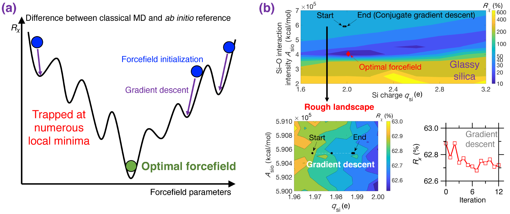

Figure 8a illustrates a cost function landscape as a function of arbitrary forcefield parameters, where the cost function R_𝜒 is defined herein as the magnitude of difference between the PDF g(r) computed by classical MD and its ab initio reference [Liu et al. 2019e]. Since the landscape is rough and features many local minima, traditional gradient-descent-based optimization algorithms are usually largely inefficient since they tend to get stuck in local minima—so that the outcome of the optimization strongly depends on the initial starting point [Shewchuk 1994].

As an illustrative example, Figure 8b shows the cost function landscape of a Buckingham forcefield for glassy silica as a function of two forcefield parameters (i.e., the silicon partial charge q_si and the short-range Si–O interaction intensity A_SiO) [Liu et al. 2019e]. Even for this simple system, the cost function landscape is rough and exhibits several local minima. As a result, optimizations relying on conjugated gradient descent [Shewchuk 1994] tend to get easily stuck at the positions nearby the start point (see Figure 8b) [Liu et al. 2019e]. Indeed, although the cost function looks fairly smooth at a high level, a closer inspection reveals that the cost function locally features a very rough landscape showing a large number of local minima (see bottom panel in Figure 8b) [Liu et al. 2019e]. Overall, as a consequence of the rough nature of typical cost function landscapes, forcefield parameterization schemes are often strongly biased, heavily relying on intuition, or requiring a large number of independent optimization (with different starting points) [Liu et al. 2019e, c].

3.2. Effect of the cooling rate

3.2.1. Importance of thermal history

Due to the short timescale that is accessible to MD simulations (up to a few nanoseconds trajectories) [Plimpton 1995a], glass simulations relying on the melt-quenching approach are limited to ultrafast cooling rates (10¹⁴–10⁹ K/s), which far exceed the cooling rates achieved in conventional experiments (10²–10⁰ K/s) [Li et al. 2017]. This is important since, glasses being out-of-equilibrium phases, their structure and properties depend on their thermal history. Specifically, glasses tend to reach deeper positions in their PEL upon decreasing cooling rates (i.e., they become more stable, see Figure 9a) [Debenedetti and Stillinger 2001].

Figure 9.
(a) Illustration of different local minimum states in the potential energy landscape (PEL) that are reached by melt-quenched glasses upon different cooling rates [Debenedetti and Stillinger 2001]. Slower cooling rates result in more stable glasses, i.e., featuring a deeper position in the PEL. (b) Evolution of the potential energy U of a glass with respect to temperature during a melt-quenching molecular dynamics (MD) simulation under fast cooling (yellow) and slow cooling (blue) [Debenedetti and Stillinger 2001]. The energy profile of a glass subjected to a melt-quenching experiment (i.e., at much lower cooling rate) is added as a reference (green). (c) Fictive temperature T_f (upper panel) and final potential energy U₀ (bottom panel) as a function of cooling rate for a (Na₂O)₃₀(SiO₂)₇₀ glass offered by both melt-quenching MD simulations (blue squares) and experiments (green squares) [Li et al. 2017; Zhou et al. 2020]. The lines are to guide the eyes.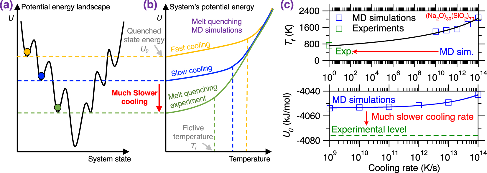

Figure 9b illustrates the evolution of the potential energy U of a glass with respect to the decreasing temperature during melt-quenching with varying cooling rates: (i) MD simulation with a large cooling rate (typically 10 K/ps), (ii) MD simulation with a slow cooling rate (typically 10⁻³ K/ps), and (iii) experimental melt-quench (typically 10⁻¹² K/ps) [Debenedetti and Stillinger 2001]. At high temperature, the three systems are at the equilibrium liquid state and, hence, exhibit the same potential energy U [Debenedetti and Stillinger 2001]. As temperature decreases, U decreases (the slope depending on the heat capacity of the liquid) and all three systems enter into the metastable supercooled liquid state following the same linear master curve [Debenedetti and Stillinger 2001]. From this point, the transition from the metastable supercooled liquid state to the out-of-equilibrium glassy state (i.e., at the glass fictive temperature T_f) occurs when the relaxation time of the system exceeds the observation time. Although, at fixed temperature, all the three systems exhibit the same relaxation time, the observation time is significantly lower in MD simulations, especially upon large cooling rate. As such, glasses simulated by MD using a large cooling rate enter the glassy state at higher temperature and remain stuck is high-energy states in the PEL (see Figures 9a and b) [Debenedetti and Stillinger 2001]. As a result, glasses simulated by MD strongly depend on the choice of the cooling rate and tend to be more stable (i.e., lower final energy U₀, more ordered) upon decreasing cooling rates.

3.2.2. Gap between simulated versus experimental glasses

Figure 9c shows the evolution of the glass fictive temperature T_f and final potential energy U₀ as a function of the cooling rate for both melt-quenching experiments and MD simulations—using the case of a (Na₂O)₃₀(SiO₂)₇₀ glass as an archetypical example [Li et al. 2017; Zhou et al. 2020]. As expected, slower cooling rates result in lower T_f and U₀. However, due to the huge gap between the cooling rates that are accessible to experiments and simulations [Li et al. 2017], experimental values of T_f and U₀ tend to be much lower than their simulation counterparts [Li et al. 2017; Zhou et al. 2020]. This difference in the order of the magnitude of the cooling rate is a critical limitation of MD simulations since it results in a systematic difference between experimental and simulated glasses [Li et al. 2017; Vollmayr et al. 1996b]. Note that different types of glasses may exhibit various dependence on the cooling rate, so that certain glasses are more sensitive to variations in the cooling rate than others [Liu et al. 2018]. It should also be noted that certain glass properties or structural features (e.g., medium-range order structure) are more sensitive to the cooling rate than others (e.g., short-range order structure) [Li et al. 2017].

3.3. Finite size effects

Figure 10.
Neutron structure factor S_N(Q) of silica glasses prepared by melt-quenching molecular dynamics (MD) simulations for varying system sizes, namely, N = 648, 5184, and 41,472 atoms [Nakano et al. 1994].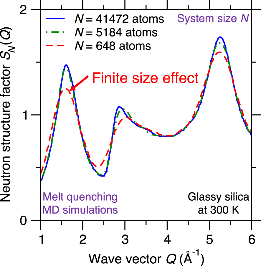

Due to their high computational cost, atomistic simulations are limited to fairly small systems (i.e., small number of atoms). Although PBC are typically used to mitigate any spurious effects arising from the presence of surfaces, the limited size of simulated glasses (from hundreds to millions of atoms) can affect the accuracy of the simulation [Du 2015]. Difficulties related to the system size include: (i) lack of statistical sampling if the number of atoms is too low [Berthier et al. 2012; Horbach et al. 1996], (ii) enhanced fluctuations in the thermodynamic properties of the simulated system (e.g., temperature or pressure) since the magnitude of fluctuations inversely scale with the square root of the number of atoms [Du 2019; Leach 2001], and (iii) systematic errors arising from the limited size of the simulation box (e.g., absence of large rings or extended collective vibrational modes) [Ganster et al. 2004; Nakano et al. 1994].

Figure 10 shows the computed neutron structure factor S_N(Q) of a glassy silica system prepared by melt-quenching MD simulations while using three different system sizes N, namely, 648 (small system), 5184 (intermediate system), and 41,472 atoms (large system) [Nakano et al. 1994]. The computed structure factor S_N(Q) is found to depend on the system size since, especially in the low-Q region (which captures the medium-range order structure of the glass)—before the structure factor eventually converges for large systems [Nakano et al. 1994]. This indicates that glass simulations relying on small simulation boxes (and, hence, small numbers of atoms) do not always properly capture the structure and properties of glasses [Du 2015; Ganster et al. 2004; Nakano et al. 1994]. In practice, one needs to select a system size that is large enough to mitigate finite size effects, but small enough to ensure a reasonable computational cost [Du 2015].

3.4. Limitations of reverse Monte Carlo (RMC) simulations

3.4.1. Need for structural data

Reverse Monte Carlo (RMC) simulations aim to construct atomistic structures that match one or several structural fingerprints provided by experiments (often, the PDF) [McGreevy 2001]. As such, RMC simulations offer an attractive alternative to MD simulations since such simulations can effectively bypass the melt-quench route to form a glass and, hence, are not affected by high cooling rate effects. However, RMC simulations largely rely on the availability (and accuracy) of experimental data. This limits the predictive power of RMC simulations since this approach does not make it possible to simulate in silico glasses that have not been experimentally synthesized and characterized yet. This also limits the range of conditions (temperature, pressure, etc.) to the ones that have already been experimentally explored.

3.4.2. Ill-defined nature of RMC simulations

Figure 11.
(a) Illustration of the existence of competitive minima in the cost function landscape for a reverse Monte Carlo (RMC) simulation [McGreevy 2001]. The cost function R_𝜒 is defined herein as the magnitude of difference between the simulated and experimental PDFs (see (1)) [Zhou et al. 2020]. Compared to the targeted minimum (green circle, which exhibits both low R_𝜒 and potential energy U), some competitive minima (red sphere) exhibit the same value of the cost function R_𝜒, but high values of U, i.e., they correspond to unstable energy states in the potential energy landscape (PEL) [Zhou et al. 2020]. (b) Illustration of atomic configurations that exhibit the same PDF g(r) while presenting notably different structures [Pandey et al. 2016b]. (c) Evolution of the cost function R_𝜒 (upper panel) and potential energy U (bottom panel) as a function of the number of Monte Carlo (MC) search steps during an RMC simulation of a sodium silicate glass ((Na₂O)₃₀(SiO₂)₇₀) [Zhou et al. 2020]. The R_𝜒 and U values obtained for the same glass prepared by melt-quenching molecular dynamics (MD) simulation with a cooling rate of 0.001 K/ps are added as references (green dash line) [Zhou et al. 2020].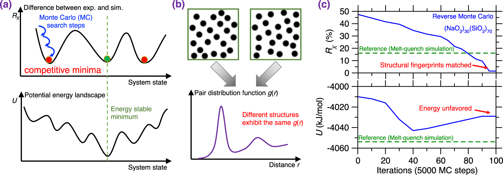

RMC simulations adopt the MC algorithm to search for an atomic structure that exhibits a minimum in the cost function landscape (see upper panel of Figure 11a) [Allen and Tildesley 2017], wherein the cost function R_𝜒 is defined as the magnitude of difference between the simulated structural fingerprints and their experimental references [Zhou et al. 2020]. This can be formulated as an optimization problem, wherein some degrees of freedom (i.e., the positions of the atoms) are adjusted so as to minimize a cost function. However, the optimization problem at the core of RMC simulations is intrinsically ill-defined. Indeed, although a given three-dimensional structure yields unique values for the fingerprints, a given fingerprint can be associated with a large number of different three-dimensional structures. That is, the structure–fingerprint relationship is not reversible. For instance, due to the complex, disordered nature of glasses [Bunde and Havlin 2012], very different structures can be associated with the same PDF (see Figure 11b) [Pandey et al. 2016b]. This is a consequence of the fact that the PDF is simply a one-dimensional signature of a glass structure (averaged over various types of elements) and, therefore, only offers a highly compressed representation of a three-dimensional structure—which does not contain enough information to robustly reconstruct the structure itself. In short, RMC simulations do not exhibit a single solution, which manifests itself by the fact that the cost function landscape exhibits various competitive minima [Pandey et al. 2015]. Since traditional RMC simulations do not embed any knowledge of the interatomic interactions, the structures generated by RMC may not be thermodynamically stable [Zhou et al. 2020] and the regions of the PEL that are explored in RMC simulations may be very different from those that are accessed during the melt-quenching of a glass (see bottom panel in Figure 11a) [Pandey et al. 2015].

Figure 11c shows the evolution of the optimization cost function R_𝜒 and the potential U with respect to the number of MC search steps during an RMC simulation for a (Na₂O)₃₀(SiO₂)₇₀ glass [Zhou et al. 2020]. Note that the values of R_𝜒 and U obtained for the same glass prepared by a melt-quenching MD simulation are also added as references [Zhou et al. 2020]. As expected, R_𝜒 gradually decreases and eventually becomes lower than the MD reference, that is, the RMC simulation offers an optimal structure that indeed matches the experimental structural fingerprints (see upper panel of Figure 11c) [Zhou et al. 2020]. However, upon RMC refinement, the potential energy U is not monotonically decreasing but, rather, tends to increase in the late stages of the MC search. Eventually, the final glass structure exhibits a notably higher potential energy U than that of the MD-simulated glass reference (see bottom panel of Figure 11c) [Zhou et al. 2020]. These results exemplify that an apparent excellent agreement with experimental data (e.g., based on the PDF) does not always translate into a realistic glass structure [Pandey et al. 2015; Zhou et al. 2020]. The ill-defined nature of RMC can be partially mitigated by the introduction of an energy penalty term U in the MC cost function to favor structures featuring low potential energy—an approach that is typically referred to as hybrid RMC [Bousige et al. 2015; Jain et al. 2006; Opletal et al. 2002]. However, hybrid RMC requires trial-and-error tests or intuition to adjust the weights of R_𝜒 and U in the cost function. In addition, hybrid RMC simulations are significantly more computationally expensive than traditional RMC simulations since the potential energy of the system U must be computed at each MC step [Zhou et al. 2020].

4. New developments in atomistic modeling of glasses

4.1. Machine-learned forcefields

4.1.1. Types of machine-learned forcefields

To address the limitations associated with empirical forcefields relying on a fixed analytical form, machine learning (ML) offers a promising pathway to develop new complex forcefields that rely on an ML model to map a given atomic configuration to its potential energy. The promise of machine-learned forcefields is to approach the accuracy of ab initio simulations with a computational burden that is more comparable to (although typically higher than) that of classical empirical forcefields. In detail, machine-learned forcefields adopt ML regression models to fit the system’s PEL as a function of the atom positions [Behler 2016; Mishin 2021; Mueller et al. 2020], without the need to rely on any physical or chemical intuition to define a functional format of the empirical forcefield [Du 2015; Huang and Kieffer 2015]. The ground-truth PEL datapoints are often provided by ab initio MD simulations [Boero et al. 2015]. Several types of regression models have been developed so far to interpolate the PEL information provided by ab initio simulations [Mishin 2021], i.e., to map the system’s atom positions {r_i} to its potential energy U{r_i} (see Figure 12a). This includes (i) physically informed neural networks (PINN) or PINN-type regression models, which use as inputs several structural features (e.g., translation- and rotation-invariant angular 3-body and radial 2-body order parameters [Bartók et al. 2013; Chmiela et al. 2018; Pun et al. 2019]) to predict the system’s potential energy U [Huan et al. 2017; Pun et al. 2019; Schütt et al. 2018], (ii) graph neural networks (GNN), which directly use as input the atom positions (modeled as a graph, wherein some nodes, the atoms, are connected by some edges, the chemical interactions) to predict U [Gilmer et al. 2017; Park et al. 2021], and (iii) Gaussian approximation potentials (GAP), which, in contrast to the neural network fitting used in PINN and GNN [Russell et al. 2010], adopt a nonparametric fitting technique (i.e., Gaussian process regression (GPR) [Rasmussen and Williams 2008]) to offer not only the PEL prediction but also the confidence interval of the prediction [Bartók et al. 2010; Bartók and Csányi 2015]. Importantly, this confidence interval can be used to train forcefields by active learning, that is, wherein new ground-truth ab initio simulations are dynamically conducted for structures associated with high confidence intervals—which are then added to the training set to retrain the GAP forcefield. Such active learning makes it possible to dynamically retrain the forcefield based on the very structures that are the most informative to improve its accuracy [Byggmästar et al. 2019; Caro 2019].

Figure 12.
(a) Schematic illustrating various methods to obtain a machine-learned forcefield by fitting the potential energy landscape (PEL) of a system through (i) physically informed neural network (PINN) [Pun et al. 2019], (ii) graph neural network (GNN) [Park et al. 2021], (iii) Gaussian approximation potential (GAP) (see text for details) [Bartók et al. 2010]. In the fitting process, the reference PEL datapoints are provided by ab initio molecular dynamics (MD) simulations [Boero et al. 2015]. (b) Example of the structural transition of amorphous silicon (a-Si) into crystalline Si when pressure increases [McMillan et al. 2005; Pandey et al. 2011], by using MD simulations relying on a machine-learned forcefield [Deringer et al. 2021]. The transition process is illustrated in terms of a PEL computed by first-principles calculation (i.e., ab initio reference [Boero et al. 2015]), machine-learned forcefield (i.e, GAP [Deringer et al. 2021]), and classical forcefield (i.e., SW potential [Stillinger and Weber 1985]), respectively. The GAP forcefield is trained by fitting the ab initio PEL datapoints (black circle) and exhibits a more accurate prediction of the transition energy of silicon upon crystallization than the classical forcefield [Deringer et al. 2021]. (c) Evolution of the average atomic volume as a function of the silicon system’s pressure using classical (i.e., SW potential [Stillinger and Weber 1985]) and machine-learned forcefields (i.e., GAP [Deringer et al. 2021]). A crystallization transition is observed using GAP (as expected) but does not occur when using the SW potential [Deringer et al. 2021].

4.1.2. Accuracy of machine-learned forcefields

As compared to empirical forcefields based on fixed functional formats [Du 2019], machine-learned forcefields exhibit more flexibility to fit the PEL and, therefore, tend to offer more accurate predictions (when properly trained) [Mishin 2021]. Figure 12b illustrates, from the viewpoint of a PEL [Lacks 2001], the amorphous-to-crystalline transition of a silicon solid upon increasing pressure [McMillan et al. 2005; Pandey et al. 2011]. The reference PEL datapoints are provided by ab initio MD simulations and are fitted by both an analytical classical and a machine-learned forcefield, respectively [Deringer et al. 2021]. The evolution of the average atomic volume as a function of pressure predicted by both the classical and machine-learned forcefields are provided in Figure 12c [Deringer et al. 2021]. On the one hand, the classical forcefield based on a SW potential offers a good description of the close-to-equilibrium states (amorphous and crystalline states, corresponding to local minima in the PEL) [Stillinger and Weber 1985], but fails to properly predict the pressure-driven amorphous-to-crystalline transition [Deringer et al. 2021] as it overestimates the energy barrier between these two states [Debenedetti and Stillinger 2001]. On the other hand, the GAP machine-learned forcefield accurately fits the reference PEL datapoints and offers an accurate prediction of the energy of the transition state upon increasing pressure [Deringer et al. 2021]. This illustrates the ability of machine-learned forcefields to offer accurate predictions, both for equilibrium and out-of-equilibrium systems [Mishin 2021]. It should nevertheless be noted that, like any ML model, the accuracy of a machine-learned forcefield largely depends on the size, accuracy, and diversity of the training set—that is, the ensemble of configurations (and their ground-truth potential energy) that are used to train the forcefield.

As an emerging family of forcefields [Chmiela et al. 2018], machine-learned forcefields have been successfully applied to simulate select glasses or disordered solids [Friederich et al. 2021], including amorphous Si [Deringer et al. 2021], silica [Li and Ando 2018], Ge–Sb–Te (GST) phase-change materials [Mocanu et al. 2020, 2018], MOFs [Eckhoff and Behler 2019], etc. On the one hand, these forcefields yield very accurate predictions, whose accuracy approaches that of ab initio MD [Chmiela et al. 2018]. On the other hand, in contrast to the high computation cost of ab initio MD [Hafner 2008], the MD simulations relying on machine-learned forcefields are more efficient, which unlocks the prediction of more complex properties—e.g., properties involving long-term timescales or extended length scales [Friederich et al. 2021], such as thermal conductivity [Sosso et al. 2018], glass reactivity [Erlebach et al. 2021], and phase transformations [Deringer et al. 2021]. Clearly, machine-learned forcefields are an extremely promising pathway to address the challenges facing the simulation of glasses, but their challenging parameterization remains a key bottleneck.

4.2. Development of analytical empirical forcefields by machine learning

4.2.1. Advantages of analytical empirical forcefields

Despite the fact that, thanks to their flexibility, machine-learned forcefields have the potential to offer very high accuracy [Mishin 2021], analytical empirical forcefields exhibit several key advantages [Du 2015; Huang and Kieffer 2015]. As an important feature, the functional forms are selected based on physical and chemical knowledge/intuition regarding the nature of the interatomic interactions [van Beest et al. 1990]. For instance, ion–ion interactions are modeled based on the Coulomb’s law, forcefields can explicitly account for Van der Waals interactions (with a term proportional to 1∕r⁶), or the dipole of an atom can explicitly be modeled as a spring in polarizable forcefields [Allen and Tildesley 2017; Carré et al. 2016; Du 2015; Fennell and Gezelter 2006; Huang and Kieffer 2015; Musgraves et al. 2019]. This tends to render empirical forcefields more physics-based, but also more interpretable than their “black-box” machine-learned counterparts [Cranmer et al. 2020; Hernandez et al. 2019]. Such fixed analytical form also has several advantages. First, it imposes a strong constraint on the predicted potential energy—for instance, the selected analytical form can ensure that the energy diverges to infinity at close distance and converges to zero at long distance [Senftle et al. 2016]. This is important as, in contrast, due to their large flexibility, machine-learned forcefields can sometimes offer unrealistic, nonphysical predictions. This is a consequence of the fact, like any ML model, machine-learned forcefields can excel at interpolating the regions of the PEL that they have been trained on, but tend to offer very unrealistic predictions far from their training set. In turn, the fixed analytical form of analytical forcefields limit their ability to accurately interpolate complex PEL, but makes them more robust and more likely to offer reasonable transferability to systems that are different from those included in the training set [Liu et al. 2019c]. Second, machine-learned forcefields typically rely on complex models (e.g., artificial neural networks) that present a very large number of tunable parameters. Such a large dimensionality must be balanced by a large training set. As a result, machine-learned forcefields typically require a significantly larger training set (that is, a larger number of configurations with their ground-truth potential energy) than analytical empirical forcefields (which typically involve orders of magnitude fewer parameters) [Liu et al. 2020a]. In addition, although machine-learned forcefields have the flexibility to interpolate any PEL without requiring any intuition regarding the nature of the interactions, they still rely on a certain number of assumptions regarding the complexity of the PEL (e.g., to determine the optimal number of neurons or layers in an artificial neural network model). Finally, although machine-learned forcefields are orders of magnitude faster than ab initio simulations, they still typically involve an increased computational burden as compared to simple analytical forcefields [Cranmer et al. 2020; Yaseen et al. 2016].

4.2.2. Machine-learning-aided parameterization scheme

Figure 13.
(a) Parameterization of a Buckingham-format empirical forcefield (see (5)) for glassy silica based on Gaussian process regression (GPR) and Bayesian optimization (BO) (see text for details) [Liu et al. 2019c]. For illustration purposes, only q_si is set as a variable, while the other forcefield parameters are fixed to their values in the well-established van Beest–Kramer–van Santen (BKS) potential [van Beest et al. 1990]. (b) Illustration of the efficient search for optimal forcefield parameters (i.e., yielding minimum R_𝜒) for glassy silica in the parameter space of the Buckingham forcefield by the iterative learning method combining GPR and BO [Liu et al. 2019e]. For illustration purposes, a two-dimensional parameter space (i.e., q_Si and A_SiO) is adopted in the search process, while the other forcefield parameters are fixed to their values in the BKS potential [van Beest et al. 1990]. The search path (white dashed line) prescribed by ML quickly identifies the optimal forcefield after only five iterations [Liu et al. 2019e].

As an alternative to machine-learned forcefields, machine-learning-aided parameterization can combine the power of ML with the robustness of analytical forcefields. Indeed, as compared to traditional gradient-descent-based parameterization schemes (see Figure 8) [Carré et al. 2016], ML offers a new paradigm to parameterize analytical forcefields in a more efficient and unbiased fashion [Liu et al. 2019e]. For instance, Figure 13 shows an ML-aided parameterization scheme based on Gaussian process regression (GPR) and Bayesian optimization (BO) [Frazier and Wang 2016; Ueno et al. 2016], which is applied to parameterize a Buckingham forcefield (see (5)) for glassy silica [Liu et al. 2019e]. The ML approach aims to find the global minimum (i.e., the optimal set of parameters) in the cost function landscape as a function of the forcefield parameters [Liu et al. 2019c], where the cost function R_𝜒 is here defined as the magnitude of difference of the PDF g(r) computed by classical MD simulation and its ab initio reference [Wright 1993].

Figure 13a illustrates the basic idea behind the use of GPR and BO to parameterize empirical forcefields [Liu et al. 2019c]. For illustration purposes, only one forcefield parameter (i.e., silicon charge q_si) is here selected to plot the cost function landscape [Liu et al. 2019c], while the other parameters are fixed to their values in the well-established BKS potential [van Beest et al. 1990]. First, the GPR model fits the known (i.e., ground-truth) points in the cost function landscape—so as to offer not only a smooth interpolation of the landscape profile but also its confidence interval (see upper panel of Figure 13a) [Liu et al. 2019c]. Then, BO prescribes the set of parameters (i.e., q_si herein) that exhibits the highest probability to yield the global minimum for R_𝜒 (see bottom panel of Figure 13a) [Liu et al. 2019c]. This is achieved by computing the expected improvement (EI) metric that offers the best balance between (i) the “exploitation” of the forcefields parameters that are predicted by the GPR model to yield a minimum R_𝜒 value and (ii) the “exploration” of the domains of forcefield parameter values that are associated with high confidence interval (i.e., high uncertainty) [Frazier and Wang 2016]. This parameterization scheme ensures that the optimal forcefield parameters (i.e., those that minimize the cost function) can quickly be identified, while mitigating the risk for the optimization scheme to remain stuck in a local minimum of the cost function landscape.

4.2.3. Efficient search of global minimum

Figure 13b shows the search path that is prescribed by ML to find the optimal forcefield parameters (i.e., those yielding a global minimum for the cost function R_𝜒) [Liu et al. 2019e]. For illustration purposes, the search is conducted within a two-dimensional parameter space (i.e., comprising the silicon partial charge q_Si and the short-range SiO interaction intensity A_SiO) [Liu et al. 2019e], while the other forcefield parameters are fixed to their values in the BKS potential [van Beest et al. 1990]. Notably, this ML-aided parameterization approach can quickly identify the optimal set of forcefield parameters after only a few iterations [Liu et al. 2019e]. Importantly, this optimization scheme is unbiased to the start position in the search space, that is, the outcome of the optimization does not depend on the initial values of the forcefield parameters [Liu et al. 2019e]. This approach offers a promising route to efficiently refine existing empirical forcefields at a fraction of the computational cost that is needed to develop a machine-learned forcefield [Liu et al. 2020a, 2019c, e].

4.3. Constructing stable glass structures by force-enhanced atomic refinement

4.3.1. Bypassing the melt-quenching route

Due to the huge gap of cooling rate between melt-quenching experiments and MD simulations (see Figure 9) [Li et al. 2017], glasses prepared by MD simulations tend to exhibit higher fictive temperature (i.e., to be less stable) than experimentally synthesized glasses [Vollmayr et al. 1996b]. Alternatively, RMC simulations can bypass this melt-quenching route by directly constructing atomic structures that match experimental data (see Section 2.2) [McGreevy 2001]. However, due to the ill-defined nature of RMC (see Section 3.4), RMC-based glasses are often thermodynamically unstable (see Figure 11) [Pandey et al. 2015; Zhou et al. 2020]. To mitigate this issue, force-enhanced atomic refinement (FEAR) has been proposed as a powerful, information-based approach that simultaneously leverages the knowledge of experimental data (which are used to constraint the glass structure) and interatomic potential (which is used to ensure the thermodynamic stability of the simulated glass) [Pandey et al. 2016a, b, 2015].

4.3.2. FEAR algorithm

Figure 14a illustrates how the FEAR algorithm searches for a realistic atomistic structure that simultaneously matches experimental data and features minimum potential energy [Pandey et al. 2016a, 2015]. In detail, each FEAR iteration consists of a given number (e.g., 5000) of RMC search steps in the cost function landscape R_𝜒 (i.e., difference between simulated and experimental data), followed by one energy minimization step in the PEL [Zhou et al. 2020]. The cost function R_𝜒 is defined herein as the magnitude of the difference between the PDFs g(r) computed by FEAR simulation and neutron diffraction experiment [Zhou et al. 2020]. RMC and energy minimalization steps are then literately repeated until both the cost function R_𝜒 and the potential energy converge. In this scheme, the RMC steps are used to slightly deform the atomic structure (so as to escape local minima in the PEL), while the energy minimization is used to ensure that the simulated structure never drifts away from the stable region of the PEL that is physically accessible [Pandey et al. 2015; Zhou et al. 2020]. Eventually, by simultaneously leveraging both experimental and interatomic energy information, FEAR simulations can yield glass structures that simultaneously exhibit enhanced agreement with available experimental data and a larger thermodynamic stability than glasses prepared by MD or RMC [Pandey et al. 2015]. It is worth pointing out that, in contrast to MD simulations that heavily rely on the accuracy of interatomic forcefields [Takada 2021], the accuracy of FEAR simulation is fairly insensitive to the quality of interatomic forcefield that is used during the energy minimization step [Zhou et al. 2021]. That is, both high- and low-quality forcefields can guide the system toward energy-stable regions in the PEL, while, eventually, the details of the simulated structure are mainly controlled by the RMC steps [Zhou et al. 2021]. Importantly, FEAR simulations are extremely computationally efficient since the potential energy of the system only needs to be computed during the energy minimization step—whereas it needs to be computed at any step during MD or hybrid RMC simulations.

4.3.3. Realistic prediction of atomistic structure

Figure 14.
(a) Illustration of the force-enhanced atomic refinement (FEAR) algorithm, which combines both Monte Carlo (MC) searches in the cost function landscape—i.e., reverse Monte Carlo (RMC) simulation [McGreevy and Pusztai 1988]—and energy minimization in the potential energy landscape (PEL) (see text for details) [Pandey et al. 2015]. (b) Evolution of the cost function R_𝜒 (see (1)) as a function of the number of optimization iterations upon RMC (blue) and FEAR simulation (green) of a sodium silicate glass ((Na₂O)₃₀(SiO₂)₇₀) [Zhou et al. 2020]. The cost function R_𝜒 of glasses prepared by melt-quenching molecular dynamics (MD) simulations at different cooling rates ranging from 10² K/ps to 10⁻³ K/ps are added as references (red dash lines) [Zhou et al. 2020]. (c) Pair distribution function (PDF) g(r) of the glasses formed at the end of the RMC, MD, and FEAR simulation [Zhou et al. 2020], compared to the g(r) reference obtained by neutron diffraction experiment [Wright et al. 1991]. (d) Evolution of the system’s potential energy U as a function of the number of optimization iterations upon RMC (blue) and FEAR simulation (green) [Zhou et al. 2020]. The potential energy of glasses prepared by melt-quenching MD simulations are also added as references (red dash lines) [Zhou et al. 2020].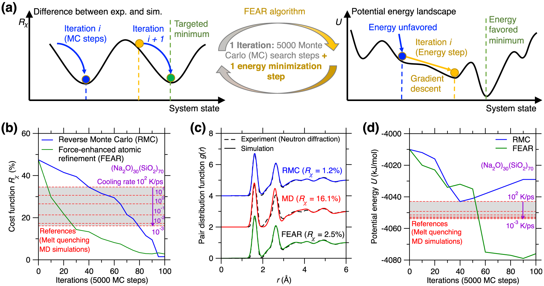

Figure 14b shows the evolution of the cost function R_𝜒 as a function of the number of optimization steps for both RMC and FEAR simulations [Zhou et al. 2020]. The R_𝜒 values of glasses prepared by melt-quenching MD simulations at different cooling rate are added as references [Zhou et al. 2020]. Both FEAR and RMC eventually offer atomistic structures exhibiting small R_𝜒 values, which are notably lower than that of the MD references [Zhou et al. 2020]. Indeed, the PDFs g(r) provided by both FEAR and RMC simulations are in excellent agreement with the experimental g(r) (see Figure 14c) [Zhou et al. 2020], while MD simulation slightly deviates from the experimental g(r) due to the large cooling rate [Li et al. 2017]. Interestingly, the energy minimizations steps upon FEAR refinement yield a faster convergence (i.e., faster decrease in the cost function R_𝜒) as compared to RMC. Further, Figure 14d shows the evolution of the potential energy U as a function of the number of optimization steps both upon FEAR and RMC simulations [Zhou et al. 2020]. MD simulation results are also added as references [Zhou et al. 2020]. It is notable that RMC simulation yields unrealistic atomic structures that are unstable as they present a potential energy that is significantly higher than those achieved by MD [Zhou et al. 2020]. In comparison, the FEAR simulation offers a notably more realistic, energy-stable atomistic structure that still satisfies the experimental constraints as well as the RMC-based structure [Zhou et al. 2020]. Importantly, the FEAR-generated structure features a potential energy that is notably lower than those achieved by melt-quenching MD, even in the case of the slowest cooling rate [Zhou et al. 2020]. This highlights the fact that the structure generated by FEAR exhibits a lower fictive temperature than the MD-based configurations—that is, FEAR can efficiently bypass limitations arising from the fast cooling rate used in MD simulations [Debenedetti and Stillinger 2001; Li et al. 2017]. This establishes FEAR as a promising technique to generate glass structures that are very stable and that can directly be quantitatively compared with experimental glasses.

5. Conclusions and future opportunities

Overall, atomistic simulations provide an efficient tool to access the atomic structure of glasses, which is otherwise challenging to directly visualize by conventional experiments. However, simulations remain plagued by a series of challenges, including (i) slow execution runtime, (ii) small accessible timescales and/or length scales, (iii) cooling rate difference between experiments and simulations, (iv) availability and accuracy of empirical forcefields, and (v) ill-defined nature of simulation protocols (e.g., RMC simulations). To overcome these limitations, one can resort to either (i) simulation protocols involving more physical information (e.g., FEAR simulations, or more accurate empirical forcefield functionals) or (ii) ML approaches (e.g., machine-learned forcefields, or ML-aided forcefield parameterization). Indeed, with the aid of ML, one can develop more accurate and computationally efficient forcefields to speed up MD simulations, thereby unlocking longer timescales or larger system sizes.

Figure 15.
Schematic summarizing future opportunities for glass modeling offered by the mutual integration of simulations and machine learning (ML). On the one hand, ML can assist in (i) developing empirical forcefields for accurate and computationally efficient simulations [Liu et al. 2019e], (ii) “separating the wheat from the chaff” in large amounts of complex simulation data to gain new insights or generate new knowledge of the underlying physics governing glasses [Liu et al. 2021b], and (iii) accelerating simulations by surrogate ML engines [Liu et al. 2021a]. On the other hand, simulation can generate large amounts of high-fidelity data that can be used to train ML models [Liu et al. 2019d], which, in turn, can be validated by simulations. Both simulations and their integration pipeline with ML can be accelerated by leveraging automated differentiable programing engines (e.g., Python JAX) and hardware accelerators (e.g., graphics processing unit (GPU) and tensor processing unit (TPU)) [Liu et al. 2020b]. Note that, when applicable, “ground-truth” experimental data can either a priori inform or a posteriori validate the physics-based (i.e., simulations) and data-based (i.e., ML) models.

As a future opportunity, we envision that smart closed-loop integrations of ML modeling and MD simulations will leapfrog glass modeling (see Figure 15). Example of such opportunities are listed in the following:

(i) Deciphering complex simulation data by ML. Atomic trajectories generated by MD simulations contains all the structural information that govern glass properties. However, due to the complex, disordered nature of glass structures, it is challenging to “separate the wheat from the chaff”, that is, to pinpoint the key structural features that govern glass properties [Tanaka et al. 2019]. In that regard, owing to its ability to discover hidden pattern in complex, multi-dimensional data, ML offers a new opportunity to identify relevant structural patterns in simulated glassy structures [Biroli 2020; Tanaka et al. 2019]. Prominent examples include the recently developed softness approach based on classification-based ML [Cubuk et al. 2017; Liu et al. 2021c, b] and graph neural networks (GNN)—a new and powerful family of ML models—that represent atomistic structures as nodes-and-edges graphs [Bapst et al. 2020]. Inputting complex simulation data into such advanced ML models makes it possible to decipher previously hidden structure–property relationships and capture the key structural features that govern glass properties. The ability to learn new physics from ML models depends on their “interpretability”. For instance, one can analyze the weight associated to each input structural feature in the softness approach [Cubuk et al. 2017; Liu et al. 2021c, b] or monitor the model responses for various graph inputs in the GNN method [Bapst et al. 2020]. These approaches make it possible to unravel the key structural patterns, that is, the ones that are the most influential in governing the properties of glasses. Finally, it is worth mentioning that, in addition to ML, topological analyzes represent an alternative, traditionally challenging but direct approach to investigate simulated glassy structures [Bauchy 2019]. For instance, some recently developed topological approaches (e.g., persistent homology [Nakamura et al. 2015]) have been demonstrated to be effective tools in identifying influential medium-range order structural features in disordered phases [Sørensen et al. 2020].

(ii) Combining simulations and ML for glasses’ inverse design. Owing to its economical nature as compared to systematic experiments, high-throughput virtual screening (HTVS, that is, the systematic simulation of a large number of glasses) offers an efficient route to identify in silico an optimal glass composition featuring an optimal characteristics within a given compositional domain [Noh et al. 2020; Sanchez-Lengeling and Aspuru-Guzik 2018]. However, although simulations excel at predicting the properties of a given glass as a function of its composition (i.e., “forward prediction”), their application to “inverse design” problems (that is, given an optimal property target, find the best glass composition) remains limited by their high computational cost—which prevents the systematic exploration of large compositional spaces [Sanchez-Lengeling and Aspuru-Guzik 2018]. To address this issue, ML offers an ideal companion to MD simulations—since an ML model can learn from a series of MD simulations and, based on this, recommend what should be the next glass composition to simulate. Such closed-loop integrations of MD and ML could greatly accelerate the discovery of novel glasses featuring desirable properties or functionalities [Liu et al. 2020b, 2019g; Noh et al. 2020]. Note that, when applicable, it is desirable to integrate experimental data into the closed loop of MD and ML, wherein such “ground-truth” experimental data can either inform or validate the models (see Figure 15). This is essential to ensure the reliability of glass modeling approaches so as to avoid any “bubble effect” arising from the error accumulation within the closed-loop integration of MD and ML (wherein MD and ML would mutually comfort and amplify each other in their improper predictions) [Bagnoli et al. 2022; Yang et al. 2019].

(iii) Leveraging differentiable programing platforms. When integrating simulations and ML models within unified pipelines, different programing languages can present a communication barrier between ML and simulation packages, which often rely on Python and C++/Fortran, respectively. In addition, most MD packages are still rooted in fairly ancient computing paradigms (e.g., with no automated differentiation), which is reminiscent of the state of ML before automatic hardware acceleration and differentiation became popular. To overcome these frictions, automatic differentiable (auto-diff) programing platforms (e.g., Python JAX [Bradbury et al. 2018]) have been recently developed to seamlessly integrate ML and simulations within unified pipelines. In contrast to traditional programing platforms that rely on handwritten derivatives (e.g., C++ [Plimpton 1995b]), auto-diff platforms excel at computing on-the-fly the backward gradient of any quantities with no additional computation burden associated with differentiation [Bradbury et al. 2018]—an operation that comes with a notable computing time in traditional simulators (e.g., force calculation in MD simulations [Allen and Tildesley 2017], see Figure 4a). Moreover, simulations built on auto-diff platforms gain backward differentiability, which makes it possible to use their outcomes to directly train ML models using gradient back propagation [Schoenholz and Cubuk 2020]. This create new opportunities to train a ML model directly based on differentiable physical knowledge rather than on data [Liu et al. 2020b]. Finally, the auto-diff platforms generally enable native “just-in-time” compilation on high-performance dedicated hardware accelerators [Bradbury et al. 2018; Schoenholz and Cubuk 2020], such as graphics processing units (GPU) and tensor processing units (TPU) [Wang et al. 2019]. Specifically, TPUs are specifically designed as matrix processors and, thanks to their tailored architecture, offer unparalleled performances in deep learning problems (up to 200X faster than GPUs). Note that MD simulations (e.g., JAX-MD [Schoenholz and Cubuk 2020]) can natively run on GPU- or TPU-based auto-diff platforms, which is key to avoid any speed bottleneck arising due to moving from one hardware to another within simulation pipelines [Plimpton 1995b; Schoenholz and Cubuk 2020]. This could greatly accelerate MD simulations relying on artificial neural networks potentials [Liu et al. 2020b; Yang et al. 2019].

(iv) Replacing slow simulations by faster surrogate ML simulation engines. Although the development of auto-diff platforms enables differentiable simulations and native hardware acceleration, the computational efficiency of numerical simulations is still limited by the intrinsic computation cost associated with the underlying numerical algorithms (e.g., Newton’s law of motion in MD simulations [Allen and Tildesley 2017]). The numerical algorithms behind scientific numerical simulations are likely to remain their bottleneck [Lane 2015; Yang et al. 2019]. To mitigate this issue, surrogate ML simulation engines offer a unique, largely untapped opportunity to replace slow simulations so as to accelerate their execution without compromising accuracy [Kochkov et al. 2021; Liu et al. 2021a]. Surrogate ML engines can be implemented as artificial neural network (ANN) models, such as convolutional neural network (CNN) [Kochkov et al. 2021] or GNN [Bapst et al. 2020].

Overall, we envision that the “fusion” of experiments, simulations, and ML models (see Figure 15) will unlock a new era in glass modeling (and materials modeling in general)—wherein traditional boundaries between physics and empirical models, knowledge and data, forward and inverse predictions, or experimental and simulation data would eventually fade. We hope that the present perspective will modestly contribute to stimulating new developments in that direction.

Conflicts of interest

Authors have no conflict of interest to declare.

Acknowledgments

This work was supported by the National Science Foundation under Grants No. CMMI-1762292, CMMI-1826420, DMR-1928538, DMREF-1922167, and CAREER-1944510. Part of this work was also supported by the Department of Energy’s Nuclear Energy University Program (DOE-NEUP: DE-NE18-15020).

Bibliographie

[Affatigato, 2015] M. Affatigato Modern Glass Characterization, John Wiley & Sons, Hoboken, NJ, 2015 | DOI

[Alder and Wainwright, 1959] B. J. Alder; T. E. Wainwright Studies in molecular dynamics. I. General method, J. Chem. Phys., Volume 31 (1959), pp. 459-466 | DOI

[Alder and Wainwright, 1960] B. J. Alder; T. E. Wainwright Studies in molecular dynamics. II. Behavior of a small number of elastic spheres, J. Chem. Phys., Volume 33 (1960), pp. 1439-1451 | DOI

[Allen and Tildesley, 2017] M. P. Allen; D. J. Tildesley Computer Simulation of Liquids, Oxford University Press, New York, 2017 | DOI

[Almeida and Santos, 2015] R. M. Almeida; L. F. Santos Raman spectroscopy of glasses, Modern Glass Characterization, John Wiley & Sons, Ltd, Hoboken, NJ, 2015, pp. 1-33 | DOI

[Andersen, 1980] H. C. Andersen Molecular dynamics simulations at constant pressure and/or temperature, J. Chem. Phys., Volume 72 (1980), pp. 2384-2393 | DOI

[Arceri et al., 2020] F. Arceri; F. P. Landes; L. Berthier; G. Biroli Glasses and aging: A statistical mechanics perspective, 2020 (cond-mat.stat-mech) | DOI

[Bachelet et al., 1982] G. B. Bachelet; D. R. Hamann; M. Schlüter Pseudopotentials that work: from H to Pu, Phys. Rev. B, Volume 26 (1982), pp. 4199-4228 | DOI

[Bagnoli et al., 2022] F. Bagnoli; G. de Bonfioli Cavalcabo; B. Casu; A. Guazzini Bubble effect induced by recommendation systems in a simple social media model, Complex Networks & Their Applications X, Studies in Computational Intelligence (R. M. Benito; C. Cherifi; H. Cherifi; E. Moro; L. M. Rocha; M. Sales-Pardo, eds.), Springer International Publishing, Cham, 2022, pp. 124-131 | DOI

[Bapst et al., 2020] V. Bapst; T. Keck; A. Grabska-Barwińska; C. Donner; E. D. Cubuk; S. S. Schoenholz; A. Obika; A. W. R. Nelson; T. Back; D. Hassabis; P. Kohli Unveiling the predictive power of static structure in glassy systems, Nat. Phys., Volume 16 (2020), pp. 448-454 | DOI

[Baral et al., 2017] K. Baral; A. Li; W.-Y. Ching Ab initio modeling of structure and properties of single and mixed alkali silicate glasses, J. Phys. Chem. A, Volume 121 (2017), pp. 7697-7708 | DOI

[Bartók and Csányi, 2015] A. P. Bartók; G. Csányi Gaussian approximation potentials: A brief tutorial introduction, Int. J. Quantum Chem., Volume 115 (2015), pp. 1051-1057 | DOI

[Bartók et al., 2010] A. P. Bartók; M. C. Payne; R. Kondor; G. Csányi Gaussian approximation potentials: the accuracy of quantum mechanics, without the electrons, Phys. Rev. Lett., Volume 104 (2010), 136403 | DOI

[Bartók et al., 2013] A. P. Bartók; R. Kondor; G. Csányi On representing chemical environments, Phys. Rev. B, Volume 87 (2013), 184115 | DOI

[Bauchy and Micoulaut, 2011] M. Bauchy; M. Micoulaut From pockets to channels: density-controlled diffusion in sodium silicates, Phys. Rev. B, Volume 83 (2011), 184118 | DOI

[Bauchy and Micoulaut, 2015] M. Bauchy; M. Micoulaut Densified network glasses and liquids with thermodynamically reversible and structurally adaptive behaviour, Nat. Commun., Volume 6 (2015), 6398 | DOI

[Bauchy et al., 2013] M. Bauchy; B. Guillot; M. Micoulaut; N. Sator Viscosity and viscosity anomalies of model silicates and magmas: a numerical investigation, Chem. Geol., Volume 346 (2013), pp. 47-56 (9th Silicate Melts Workshop) | DOI

[Bauchy et al., 2015] M. Bauchy; H. Laubie; M. J. Abdolhosseini Qomi; C. G. Hoover; F.-J. Ulm; R. J.-M. Pellenq Fracture toughness of calcium–silicate–hydrate from molecular dynamics simulations, J. Non Cryst. Solids, Volume 419 (2015), pp. 58-64 | DOI

[Bauchy et al., 2016] M. Bauchy; B. Wang; M. Wang; Y. Yu; M. J. Abdolhosseini Qomi; M. M. Smedskjaer; C. Bichara; F.-J. Ulm; R. Pellenq Fracture toughness anomalies: viewpoint of topological constraint theory, Acta Mater., Volume 121 (2016), pp. 234-239 | DOI

[Bauchy et al., 2017] M. Bauchy; M. Wang; Y. Yu; B. Wang; N. M. A. Krishnan; E. Masoero; F.-J. Ulm; R. Pellenq Topological control on the structural relaxation of atomic networks under stress, Phys. Rev. Lett., Volume 119 (2017), 035502 | DOI

[Bauchy, 2012] M. Bauchy Structural, vibrational, and thermal properties of densified silicates: Insights from molecular dynamics, J. Chem. Phys., Volume 137 (2012), 044510 | DOI

[Bauchy, 2014] M. Bauchy Structural, vibrational, and elastic properties of a calcium aluminosilicate glass from molecular dynamics simulations: The role of the potential, J. Chem. Phys., Volume 141 (2014), 024507 | DOI

[Bauchy, 2019] M. Bauchy Deciphering the atomic genome of glasses by topological constraint theory and molecular dynamics: A review, Comput. Mater. Sci., Volume 159 (2019), pp. 95-102 | DOI

[Beake et al., 2013] E. O. R. Beake; M. T. Dove; A. E. Phillips; D. A. Keen; M. G. Tucker; A. L. Goodwin; T. D. Bennett; A. K. Cheetham Flexibility of zeolitic imidazolate framework structures studied by neutron total scattering and the reverse Monte Carlo method, J. Phys. Condens. Matter, Volume 25 (2013), 395403 | DOI

[Behler, 2016] J. Behler Perspective: Machine learning potentials for atomistic simulations, J. Chem. Phys., Volume 145 (2016), 170901 | DOI

[Berthier and Ediger, 2020] L. Berthier; M. D. Ediger How to “measure” a structural relaxation time that is too long to be measured?, J. Chem. Phys., Volume 153 (2020), 044501 | DOI

[Berthier et al., 2012] L. Berthier; G. Biroli; D. Coslovich; W. Kob; C. Toninelli Finite-size effects in the dynamics of glass-forming liquids, Phys. Rev. E, Volume 86 (2012), 031502 | DOI

[Binder and Kob, 2011] K. Binder; W. Kob Glassy Materials and Disordered Solids: An Introduction to Their Statistical Mechanics, World Scientific, Singapore, 2011 | DOI

[Biroli, 2020] G. Biroli Machine learning glasses, Nat. Phys., Volume 16 (2020), pp. 373-374 | DOI

[Biswas et al., 2004] P. Biswas; R. Atta-Fynn; D. A. Drabold Reverse Monte Carlo modeling of amorphous silicon, Phys. Rev. B, Volume 69 (2004), 195207 | DOI

[Bitzek et al., 2006] E. Bitzek; P. Koskinen; F. Gähler; M. Moseler; P. Gumbsch Structural relaxation made simple, Phys. Rev. Lett., Volume 97 (2006), 170201 | DOI

[Boero et al., 2015] M. Boero; A. Bouzid; S. Le Roux; B. Ozdamar; C. Massobrio First-principles molecular dynamics methods: an overview, Molecular Dynamics Simulations of Disordered Materials, Springer Series in Materials Science (C. Massobrio; J. Du; M. Bernasconi; P. S. Salmon, eds.), Springer International Publishing, Cham, 2015, pp. 33-55 | DOI

[Bottaro and Lindorff-Larsen, 2018] S. Bottaro; K. Lindorff-Larsen Biophysical experiments and biomolecular simulations: a perfect match?, Science, Volume 361 (2018), pp. 355-360 | DOI

[Bouhadja et al., 2013] M. Bouhadja; N. Jakse; A. Pasturel Structural and dynamic properties of calcium aluminosilicate melts: a molecular dynamics study, J. Chem. Phys., Volume 138 (2013), 224510 | DOI

[Bousige et al., 2015] C. Bousige; A. Boţan; F.-J. Ulm; R. J.-M. Pellenq; B. Coasne Optimized molecular reconstruction procedure combining hybrid reverse Monte Carlo and molecular dynamics, J. Chem. Phys., Volume 142 (2015), 114112 | DOI

[Bouty et al., 2014] O. Bouty; J. M. Delaye; B. Beuneu; T. Charpentier Modelling borosilicate glasses of nuclear interest with the help of RMC, WAXS, neutron diffraction and 11B NMR, J. Non Cryst. Solids, Volume 401 (2014), pp. 27-31 STRUCTURE OF NON-CRYSTALLINE MATERIALS 12 Proceedings of the 12th International Conference on the Structure of Non-Crystalline Materials (NCM 12) | DOI

[Bradbury et al., 2018] J. Bradbury; R. Frostig; P. Hawkins; M. J. Johnson; C. Leary; D. Maclaurin; G. Necula; A. Paszke; J. VanderPlas; S. Wanderman-Milne; Q. Zhang JAX: composable transformations of Python+NumPy programs, 2018 http://github.com/google/jax

[Buehler et al., 2006] M. J. Buehler; A. C. T. van Duin; W. A. Goddard Multiparadigm modeling of dynamical crack propagation in silicon using a reactive force field, Phys. Rev. Lett., Volume 96 (2006), 095505 | DOI

[Bunde and Havlin, 2012] A. Bunde; S. Havlin Fractals and Disordered Systems, Springer Science & Business Media, Berlin, Heidelberg, 2012

[Byggmästar et al., 2019] J. Byggmästar; A. Hamedani; K. Nordlund; F. Djurabekova Machine-learning interatomic potential for radiation damage and defects in tungsten, Phys. Rev. B, Volume 100 (2019), 144105 | DOI

[Car and Parrinello, 1985] R. Car; M. Parrinello Unified approach for molecular dynamics and density-functional theory, Phys. Rev. Lett., Volume 55 (1985), pp. 2471-2474 | DOI

[Car and Parrinello, 1988] R. Car; M. Parrinello Structural, dymanical, and electronic properties of amorphous silicon: an ab initio molecular-dynamics study, Phys. Rev. Lett., Volume 60 (1988), pp. 204-207 | DOI

[Caravati et al., 2009] S. Caravati; M. Bernasconi; T. D. Kühne; M. Krack; M. Parrinello First-principles study of crystalline and amorphous Ge $_{2}$ Sb $_{2}$ Te $_{5}$ and the effects of stoichiometric defects, J. Phys. Condens. Matter, Volume 21 (2009), 255501 | DOI

[Caro, 2019] M. A. Caro Optimizing many-body atomic descriptors for enhanced computational performance of machine learning based interatomic potentials, Phys. Rev. B, Volume 100 (2019), 024112 | DOI

[Carré et al., 2007] A. Carré; L. Berthier; J. Horbach; S. Ispas; W. Kob Amorphous silica modeled with truncated and screened Coulomb interactions: a molecular dynamics simulation study, J. Chem. Phys., Volume 127 (2007), 114512 | DOI

[Carré et al., 2008] A. Carré; J. Horbach; S. Ispas; W. Kob New fitting scheme to obtain effective potential from Car-Parrinello molecular-dynamics simulations: Application to silica, Europhys. Lett., Volume 82 (2008), 17001 | DOI

[Carré et al., 2016] A. Carré; S. Ispas; J. Horbach; W. Kob Developing empirical potentials from ab initio simulations: the case of amorphous silica, Comput. Mater. Sci., Volume 124 (2016), pp. 323-334 | DOI

[Chialvo and Debenedetti, 1990] A. A. Chialvo; P. G. Debenedetti On the use of the Verlet neighbor list in molecular dynamics, Comput. Phys. Commun., Volume 60 (1990), pp. 215-224 | DOI

[Chmiela et al., 2018] S. Chmiela; H. E. Sauceda; K.-R. Müller; A. Tkatchenko Towards exact molecular dynamics simulations with machine-learned force fields, Nat. Commun., Volume 9 (2018), pp. 1-10 | DOI

[Christensen et al., 2021] R. Christensen; S. S. Sørensen; H. Liu; K. Li; M. Bauchy; M. M. Smedskjaer Interatomic potential parameterization using particle swarm optimization: case study of glassy silica, J. Chem. Phys., Volume 154 (2021), 134505 | DOI

[Cobb et al., 1996] M. Cobb; D. A. Drabold; R. L. Cappelletti Ab initio molecular-dynamics study of the structural, vibrational, and electronic properties of glassy GeSe $_{2}$ , Phys. Rev. B, Volume 54 (1996), pp. 12162-12171 | DOI

[Cormack and Du, 2001] A. N. Cormack; J. Du Molecular dynamics simulations of soda–lime–silicate glasses, J. Non Cryst. Solids, Volume 293–295 (2001), pp. 283-289 (8th Int. Conf. on Non-Crystalline Materials) | DOI

[Cormack et al., 2002] A. N. Cormack; J. Du; T. R. Zeitler Alkali ion migration mechanisms in silicate glasses probed by molecular dynamics simulations, Phys. Chem. Chem. Phys., Volume 4 (2002), pp. 3193-3197 | DOI

[Cormier et al., 2003] L. Cormier; D. Ghaleb; D. R. Neuville; J.-M. Delaye; G. Calas Chemical dependence of network topology of calcium aluminosilicate glasses: a computer simulation study, J. Non Cryst. Solids, Volume 332 (2003), pp. 255-270 | DOI

[Cranmer et al., 2020] M. Cranmer; A. Sanchez-Gonzalez; P. Battaglia; R. Xu; K. Cranmer; D. Spergel; S. Ho, 34th Conference on Neural Information Processing Systems (NeurIPS 2020), Vancouver, Canada (2020)

[Cubuk et al., 2017] E. D. Cubuk; R. J. S. Ivancic; S. S. Schoenholz; D. J. Strickland; A. Basu; Z. S. Davidson; J. Fontaine; J. L. Hor; Y.-R. Huang; Y. Jiang; N. C. Keim; K. D. Koshigan; J. A. Lefever; T. Liu; X.-G. Ma; D. J. Magagnosc; E. Morrow; C. P. Ortiz; J. M. Rieser; A. Shavit; T. Still; Y. Xu; Y. Zhang; K. N. Nordstrom; P. E. Arratia; R. W. Carpick; D. J. Durian; Z. Fakhraai; D. J. Jerolmack; D. Lee; J. Li; R. Riggleman; K. T. Turner; A. G. Yodh; D. S. Gianola; A. J. Liu Structure-property relationships from universal signatures of plasticity in disordered solids, Science, Volume 358 (2017), pp. 1033-1037 | DOI

[Darby et al., 2020] J. P. Darby; M. Arhangelskis; A. D. Katsenis; J. M. Marrett; T. Friščić; A. J. Morris Ab initio prediction of metal-organic framework structures, Chem. Mater., Volume 32 (2020), pp. 5835-5844 | DOI

[Daw and Baskes, 1983] M. S. Daw; M. I. Baskes Semiempirical, quantum mechanical calculation of hydrogen embrittlement in metals, Phys. Rev. Lett., Volume 50 (1983), pp. 1285-1288 | DOI

[Daw and Baskes, 1984] M. S. Daw; M. I. Baskes Embedded-atom method: derivation and application to impurities, surfaces, and other defects in metals, Phys. Rev. B, Volume 29 (1984), pp. 6443-6453 | DOI

[Daw et al., 1993] M. S. Daw; S. M. Foiles; M. I. Baskes The embedded-atom method: a review of theory and applications, Mater. Sci. Rep., Volume 9 (1993), pp. 251-310 | DOI

[Debenedetti and Stillinger, 2001] P. G. Debenedetti; F. H. Stillinger Supercooled liquids and the glass transition, Nature, Volume 410 (2001), pp. 259-267 | DOI

[Deng et al., 2019] L. Deng; K. Miyatani; S. Amma; M. Suehara; M. Ono; Y. Yamamoto; S. Urata; J. Du Reaction mechanisms and interfacial behaviors of sodium silicate glass in an aqueous environment from reactive force field-based molecular dynamics simulations, J. Phys. Chem. C, Volume 123 (2019), pp. 21538-21547 | DOI

[Deng et al., 2020] L. Deng; S. Urata; Y. Takimoto; T. Miyajima; S. H. Hahn; A. C. T. Duin; J. van Structural features of sodium silicate glasses from reactive force field-based molecular dynamics simulations, J. Am. Ceram. Soc., Volume 103 (2020), pp. 1600-1614 | DOI

[Deng et al., 2021] L. Deng; K. Miyatani; M. Suehara; S. Amma; M. Ono; S. Urata; J. Du Ion-exchange mechanisms and interfacial reaction kinetics during aqueous corrosion of sodium silicate glasses, NPJ Mater. Degrad., Volume 5 (2021), pp. 1-13 | DOI

[Deringer et al., 2021] V. L. Deringer; N. Bernstein; G. Csányi; C. B. Mahmoud; M. Ceriotti; M. Wilson; D. A. Drabold; S. R. Elliott Origins of structural and electronic transitions in disordered silicon, Nature, Volume 589 (2021), pp. 59-64 | DOI

[Ding and Andersen, 1986] K. Ding; H. C. Andersen Molecular-dynamics simulation of amorphous germanium, Phys. Rev. B, Volume 34 (1986), pp. 6987-6991 | DOI

[Dongol et al., 2018] R. Dongol; L. Wang; A. N. Cormack; S. K. Sundaram Molecular dynamics simulation of sodium aluminosilicate glass structures and glass surface-water reactions using the reactive force field (ReaxFF), Appl. Surf. Sci., Volume 439 (2018), pp. 1103-1110 | DOI

[Du and Cormack, 2004] J. Du; A. N. Cormack The medium range structure of sodium silicate glasses: a molecular dynamics simulation, J. Non Cryst. Solids, Volume 349 (2004), pp. 66-79 (Glass Science for High Technology. 16th University Conference on Glass Science) | DOI

[Du and Corrales, 2006] J. Du; L. R. Corrales Compositional dependence of the first sharp diffraction peaks in alkali silicate glasses: A molecular dynamics study, J. Non Cryst. Solids, Volume 352 (2006), pp. 3255-3269 | DOI

[Du et al., 2018] T. Du; H. Li; G. Sant; M. Bauchy New insights into the sol–gel condensation of silica by reactive molecular dynamics simulations, J. Chem. Phys., Volume 148 (2018), 234504 | DOI

[Du et al., 2019a] T. Du; H. Li; Q. Zhou; Z. Wang; G. Sant; J. V. Ryan; M. Bauchy Atomistic origin of the passivation effect in hydrated silicate glasses, NPJ Mater. Degrad., Volume 3 (2019a), 6 | DOI

[Du et al., 2019b] T. Du; H. Li; Q. Zhou; Z. Wang; G. Sant; J. V. Ryan; M. Bauchy Chemical composition of calcium-silicate-hydrate gels: Competition between kinetics and thermodynamics, Phys. Rev. Mater., Volume 3 (2019b), 065603 | DOI

[Du, 2015] J. Du Challenges in molecular dynamics simulations of multicomponent oxide glasses, Molecular Dynamics Simulations of Disordered Materials: From Network Glasses to Phase-Change Memory Alloys, Springer Series in Materials Science (C. Massobrio; J. Du; M. Bernasconi; P. S. Salmon, eds.), Springer International Publishing, Cham, 2015, pp. 157-180 | DOI

[Du, 2019] J. Du Molecular dynamics simulations of oxide glasses, Springer Handbook of Glass, Springer Handbooks (J. D. Musgraves; J. Hu; L. Calvez, eds.), Springer International Publishing, Cham, 2019, pp. 1131-1155 | DOI

[Durandurdu and Drabold, 2002] M. Durandurdu; D. A. Drabold Simulation of pressure-induced polyamorphism in a chalcogenide glass GeSe $_{2}$ , Phys. Rev. B, Volume 65 (2002), 104208 | DOI

[Eckhoff and Behler, 2019] M. Eckhoff; J. Behler From molecular fragments to the bulk: development of a neural network potential for MOF-5, J. Chem. Theory Comput., Volume 15 (2019), pp. 3793-3809 | DOI

[Erlebach et al., 2021] A. Erlebach; P. Nachtigall; L. Grajciar Accurate large-scale simulations of siliceous zeolites by neural network potentials, 2021 ([cond-mat.mtrl-sci]) | DOI

[Ewald, 1921] P. Ewald Evaluation of optical and electrostatic lattice potentials, Ann. Phys., Volume 64 (1921), pp. 253-287

[Fennell and Gezelter, 2006] C. J. Fennell; J. D. Gezelter Is the Ewald summation still necessary? Pairwise alternatives to the accepted standard for long-range electrostatics, J. Chem. Phys., Volume 124 (2006), 234104 | DOI

[Fernandez-Martinez et al., 2013] A. Fernandez-Martinez; B. Kalkan; S. M. Clark; G. A. Waychunas Pressure-induced polyamorphism and formation of ‘aragonitic’ amorphous calcium carbonate, Angew. Chem., Volume 125 (2013), pp. 8512-8515 | DOI

[Fischer et al., 2005] H. E. Fischer; A. C. Barnes; P. S. Salmon Neutron and x-ray diffraction studies of liquids and glasses, Rep. Prog. Phys., Volume 69 (2005), pp. 233-299 | DOI

[Fogarty et al., 2010] J. C. Fogarty; H. M. Aktulga; A. Y. Grama; A. C. T. Duin; S. A. van Pandit A reactive molecular dynamics simulation of the silica-water interface, J. Chem. Phys., Volume 132 (2010), 174704 | DOI

[Frazier and Wang, 2016] P. I. Frazier; J. Wang Bayesian optimization for materials design, Information Science for Materials Discovery and Design, Springer Series in Materials Science, Springer, Cham, 2016, pp. 45-75 | DOI

[Friederich et al., 2021] P. Friederich; F. Häse; J. Proppe; A. Aspuru-Guzik Machine-learned potentials for next-generation matter simulations, Nat. Mater., Volume 20 (2021), pp. 750-761 | DOI

[Fulde, 1995] P. Fulde Electron Correlations in Molecules and Solids, Springer Science & Business Media, Berlin, Heidelberg, 1995 | DOI

[Fullerton and Berthier, 2020] C. J. Fullerton; L. Berthier Glassy behavior of sticky spheres: what lies beyond experimental timescales?, Phys. Rev. Lett., Volume 125 (2020), 258004 | DOI

[Gaillac et al., 2017] R. Gaillac; P. Pullumbi; K. A. Beyer; K. W. Chapman; D. A. Keen; T. D. Bennett; F.-X. Coudert Liquid metal–organic frameworks, Nat. Mater., Volume 16 (2017) | DOI

[Ganster et al., 2004] P. Ganster; M. Benoit; W. Kob; J.-M. Delaye Structural properties of a calcium aluminosilicate glass from molecular-dynamics simulations: A finite size effects study, J. Chem. Phys., Volume 120 (2004), pp. 10172-10181 | DOI

[Ganster et al., 2007] P. Ganster; M. Benoit; J.-M. Delaye; W. Kob Structural and vibrational properties of a calcium aluminosilicate glass: classical force-fields vs. first-principles, Mol. Simul., Volume 33 (2007), pp. 1093-1103 | DOI

[Gilmer et al., 2017] J. Gilmer; S. S. Schoenholz; P. F. Riley; O. Vinyals; G. E. Dahl, International Conference on Machine Learning. Presented at the International Conference on Machine Learning, PMLR, Sydney, Australia (2017), pp. 1263-1272

[Goldstein, 1969] M. Goldstein Viscous liquids and the glass transition: a potential energy barrier picture, J. Chem. Phys., Volume 51 (1969), pp. 3728-3739 | DOI

[Goodwin et al., 2010] A. L. Goodwin; F. M. Michel; B. L. Phillips; D. A. Keen; M. T. Dove; R. J. Reeder Nanoporous structure and medium-range order in synthetic amorphous calcium carbonate, Chem. Mater., Volume 22 (2010), pp. 3197-3205 | DOI

[Greaves and Sen, 2007] G. N. Greaves; S. Sen Inorganic glasses, glass-forming liquids and amorphizing solids, Adv. Phys., Volume 56 (2007), pp. 1-166 | DOI

[Grigoriev et al., 2016] F. V. Grigoriev; E. V. Katkova; A. V. Sulimov; V. B. Sulimov; A. V. Tikhonravov Annealing of deposited SiO $_{2}$ thin films: full-atomistic simulation results, Opt. Mater. Express, OME, Volume 6 (2016), pp. 3960-3966 | DOI

[Grimley et al., 1990] D. I. Grimley; A. C. Wright; R. N. Sinclair Neutron scattering from vitreous silica IV. Time-of-flight diffraction, J. Non Cryst. Solids, Volume 119 (1990), pp. 49-64 | DOI

[Grubmüller et al., 1991] H. Grubmüller; H. Heller; A. Windemuth; K. Schulten Generalized verlet algorithm for efficient molecular dynamics simulations with long-range interactions, Mol. Simul., Volume 6 (1991), pp. 121-142 | DOI

[Gunnarsson and Jones, 1985] O. Gunnarsson; R. O. Jones Total-energy differences: sources of error in local-density approximations, Phys. Rev. B, Volume 31 (1985), pp. 7588-7602 | DOI

[Hafner, 2008] J. Hafner Ab-initio simulations of materials using VASP: density-functional theory and beyond, J. Comput. Chem., Volume 29 (2008), pp. 2044-2078 | DOI

[Hamann et al., 1979] D. R. Hamann; M. Schlüter; C. Chiang Norm-conserving pseudopotentials, Phys. Rev. Lett., Volume 43 (1979), pp. 1494-1497 | DOI

[Hernandez et al., 2019] A. Hernandez; A. Balasubramanian; F. Yuan; S. A. M. Mason; T. Mueller Fast, accurate, and transferable many-body interatomic potentials by symbolic regression, NPJ Comput. Mater., Volume 5 (2019), 112 | DOI

[Hockney and Eastwood, 1988] R. W. Hockney; J. W. Eastwood Computer Simulation Using Particles, Taylor & Francis Group, New York, 1988 | DOI

[Hohenberg and Kohn, 1964] P. Hohenberg; W. Kohn Inhomogeneous electron gas, Phys. Rev., Volume 136 (1964), p. B864-B871 | DOI

[Hoover, 1985] W. G. Hoover Canonical dynamics: equilibrium phase-space distributions, Phys. Rev. A, Volume 31 (1985), pp. 1695-1697 | DOI

[Horbach et al., 1996] J. Horbach; W. Kob; K. Binder; C. A. Angell Finite size effects in simulations of glass dynamics, Phys. Rev. E, Volume 54 (1996), p. R5897-R5900 | DOI

[Huan et al., 2017] T. D. Huan; R. Batra; J. Chapman; S. Krishnan; L. Chen; R. Ramprasad A universal strategy for the creation of machine learning-based atomistic force fields, NPJ Comput. Mater., Volume 3 (2017), 37 | DOI

[Huang and Kieffer, 2015] L. Huang; J. Kieffer Challenges in modeling mixed ionic-covalent glass formers, Molecular Dynamics Simulations of Disordered Materials: From Network Glasses to Phase-Change Memory Alloys, Springer Series in Materials Science (C. Massobrio; J. Du; M. Bernasconi; P. S. Salmon, eds.), Springer International Publishing, Cham, 2015, pp. 87-112 | DOI

[Huang et al., 2013] P. Y. Huang; S. Kurasch; J. S. Alden; A. Shekhawat; A. A. Alemi; P. L. McEuen; J. P. Sethna; U. Kaiser; D. A. Muller Imaging atomic rearrangements in two-dimensional silica glass: watching Silica’s dance, Science, Volume 342 (2013), pp. 224-227 | DOI

[Ispas et al., 2002] S. Ispas; M. Benoit; P. Jund; R. Jullien Structural properties of glassy and liquid sodium tetrasilicate: comparison between ab initio and classical molecular dynamics simulations, J. Non Cryst. Solids, Volume 307–310 (2002), pp. 946-955 | DOI

[Iype et al., 2013] E. Iype; M. Hütter; A. P. J. Jansen; S. V. Nedea; C. C. M. Rindt Parameterization of a reactive force field using a Monte Carlo algorithm, J. Comput. Chem., Volume 34 (2013), pp. 1143-1154 | DOI

[Jahn and Madden, 2007] S. Jahn; P. A. Madden Modeling earth materials from crustal to lower mantle conditions: a transferable set of interaction potentials for the CMAS system, Phys. Earth Plane. Inter., Volume 162 (2007), pp. 129-139 | DOI

[Jahn et al., 2006] S. Jahn; P. A. Madden; M. Wilson Transferable interaction model for Al $_{2}$ O $_{3}$ , Phys. Rev. B, Volume 74 (2006), 024112 | DOI

[Jain et al., 2006] S. K. Jain; R. J.-M. Pellenq; J. P. Pikunic; K. E. Gubbins Molecular modeling of porous carbons using the hybrid reverse Monte Carlo method, Langmuir, Volume 22 (2006), pp. 9942-9948 | DOI

[Johnson et al., 1993] B. G. Johnson; P. M. W. Gill; J. A. Pople The performance of a family of density functional methods, J. Chem. Phys., Volume 98 (1993), pp. 5612-5626 | DOI

[Kamitsos, 2015] E. I. Kamitsos Infrared spectroscopy of glasses, Modern Glass Characterization, John Wiley & Sons, Ltd, Hoboken, NJ, 2015, pp. 1-42

[Keen and McGreevy, 1990] D. A. Keen; R. L. McGreevy Structural modelling of glasses using reverse Monte Carlo simulation, Nature, Volume 344 (1990), pp. 423-425 | DOI

[Kieu et al., 2011] L.-H. Kieu; J.-M. Delaye; L. Cormier; C. Stolz Development of empirical potentials for sodium borosilicate glass systems, J. Non Cryst. Solids, Volume 357 (2011), pp. 3313-3321 | DOI

[Kochkov et al., 2021] D. Kochkov; J. A. Smith; A. Alieva; Q. Wang; M. P. Brenner; S. Hoyer Machine learning accelerated computational fluid dynamics, Proc. Natl. Acad. Sci. USA, Volume 118 (2021) no. 21, 2101784118 | DOI

[Kohn and Sham, 1965] W. Kohn; L. J. Sham Self-consistent equations including exchange and correlation effects, Phys. Rev., Volume 140 (1965), p. A1133-A1138 | DOI

[Krishnan et al., 2017a] N. M. A. Krishnan; B. Wang; Y. Yu; Y. Le Pape; G. Sant; M. Bauchy Enthalpy landscape dictates the irradiation-induced disordering of quartz, Phys. Rev. X, Volume 7 (2017a), 031019 | DOI

[Krishnan et al., 2017b] N. M. A. Krishnan; B. Wang; Y. Le Pape; G. Sant; M. Bauchy Irradiation- vs. vitrification-induced disordering: The case of $α$ -quartz and glassy silica, J. Chem. Phys., Volume 146 (2017b), 204502 | DOI

[Krishnan et al., 2017c] N. M. A. Krishnan; B. Wang; G. Sant; J. C. Phillips; M. Bauchy Revealing the effect of irradiation on cement hydrates: evidence of a topological self-organization, ACS Appl. Mater. Interfaces, Volume 9 (2017c), pp. 32377-32385 | DOI

[Kroeker, 2015] S. Kroeker Nuclear magnetic resonance spectroscopy of glasses, Modern Glass Characterization, John Wiley & Sons, Ltd, Hoboken, NJ, 2015, pp. 1-30 | DOI

[Lacks and Osborne, 2004] D. J. Lacks; M. J. Osborne Energy landscape picture of overaging and rejuvenation in a sheared glass, Phys. Rev. Lett., Volume 93 (2004), 255501 | DOI

[Lacks, 2001] D. J. Lacks Energy landscapes and the non-newtonian viscosity of liquids and glasses, Phys. Rev. Lett., Volume 87 (2001), 225502 | DOI

[Lane, 2015] J. M. D. Lane Cooling rate and stress relaxation in silica melts and glasses via microsecond molecular dynamics, Phys. Rev. E, Volume 92 (2015), 012320 | DOI

[Langreth and Mehl, 1983] D. C. Langreth; M. J. Mehl Beyond the local-density approximation in calculations of ground-state electronic properties, Phys. Rev. B, Volume 28 (1983), pp. 1809-1834 | DOI

[Leach, 2001] A. R. Leach Molecular Modelling: Principles and Applications, Prentice Hall, New York, 2001

[Levchenko et al., 2020] Theory and Simulation in Physics for Materials Applications: Cutting-Edge Techniques in Theoretical and Computational Materials Science, Springer Series in Materials Science (E. V. Levchenko; Y. J. Dappe; G. Ori, eds.), Springer International Publishing, Cham, 2020 | DOI

[Leven et al., 2021] I. Leven; H. Hao; S. Tan; X. Guan; K. A. Penrod; D. Akbarian; B. Evangelisti; M. J. Hossain; M. M. Islam; J. P. Koski; S. Moore; H. M. Aktulga; A. C. T. van Duin; T. Head-Gordon Recent advances for improving the accuracy, transferability, and efficiency of reactive force fields, J. Chem. Theory Comput., Volume 17 (2021), pp. 3237-3251 | DOI

[Levesque and Verlet, 1993] D. Levesque; L. Verlet Molecular dynamics and time reversibility, J. Stat. Phys., Volume 72 (1993), pp. 519-537 | DOI

[Le Losq et al., 2017] C. Le Losq; D. R. Neuville; W. Chen; P. Florian; D. Massiot; Z. Zhou; G. N. Greaves Percolation channels: a universal idea to describe the atomic structure and dynamics of glasses and melts, Sci. Rep., Volume 7 (2017), 16490 | DOI

[Li and Ando, 2018] W. Li; Y. Ando Comparison of different machine learning models for the prediction of forces in copper and silicon dioxide, Phys. Chem. Chem. Phys., Volume 20 (2018), pp. 30006-30020 | DOI

[Li et al., 2017] X. Li; W. Song; K. Yang; N. M. A. Krishnan; B. Wang; M. M. Smedskjaer; J. C. Mauro; G. Sant; M. Balonis; M. Bauchy Cooling rate effects in sodium silicate glasses: bridging the gap between molecular dynamics simulations and experiments, J. Chem. Phys., Volume 147 (2017), 074501 | DOI

[Liu et al., 2018] Z. Liu; Y. Hu; X. Li; W. Song; S. Goyal; M. Micoulaut; M. Bauchy Glass relaxation and hysteresis of the glass transition by molecular dynamics simulations, Phys. Rev. B, Volume 98 (2018), 104205 | DOI

[Liu et al., 2019a] H. Liu; S. Dong; N. M. A. Krishnan; E. Masoero; G. Sant; M. Bauchy Long-term creep deformations in colloidal calcium–silicate–hydrate gels by accelerated aging simulations, J. Colloid Interface Sci., Volume 542 (2019a), pp. 339-346 | DOI

[Liu et al., 2019b] H. Liu; S. Dong; L. Tang; N. M. A. Krishnan; G. Sant; M. Bauchy Effects of polydispersity and disorder on the mechanical properties of hydrated silicate gels, J. Mech. Phys. Solids, Volume 122 (2019b), pp. 555-565 | DOI

[Liu et al., 2019c] H. Liu; Z. Fu; Y. Li; N. F. A. Sabri; M. Bauchy Balance between accuracy and simplicity in empirical forcefields for glass modeling: insights from machine learning, J. Non Cryst. Solids, Volume 515 (2019c), pp. 133-142 | DOI

[Liu et al., 2019d] H. Liu; Z. Fu; K. Yang; X. Xu; M. Bauchy Machine learning for glass science and engineering: a review, J. Non Cryst. Solids, Volume 4 (2019d), 100036 | DOI

[Liu et al., 2019e] H. Liu; Z. Fu; K. Yang; X. Xu; M. Bauchy Parameterization of empirical forcefields for glassy silica using machine learning, MRS Commun., Volume 9 (2019e), pp. 593-599 (article no. mrc.2019.47) | DOI

[Liu et al., 2019f] H. Liu; L. Tang; N. M. A. Krishnan; G. Sant; M. Bauchy Structural percolation controls the precipitation kinetics of colloidal calcium–silicate–hydrate gels, J. Phys. D: Appl. Phys., Volume 52 (2019f), 315301 | DOI

[Liu et al., 2019g] H. Liu; T. Zhang; N. M. A. Krishnan; M. M. Smedskjaer; J. V. Ryan; S. Gin; M. Bauchy Predicting the dissolution kinetics of silicate glasses by topology-informed machine learning, NPJ Mater. Degrad., Volume 3 (2019g), pp. 1-12 | DOI

[Liu et al., 2020a] Han Liu; Y. Li; Z. Fu; K. Li; M. Bauchy Exploring the landscape of Buckingham potentials for silica by machine learning: soft vs hard interatomic forcefields, J. Chem. Phys., Volume 152 (2020a), 051101 | DOI

[Liu et al., 2020b] Han Liu; Y. Liu; Z. Zhao; M. Bauchy; S. S. Schoenholz; E. D. Cubuk End-to-End Differentiability and Tensor Processing Unit Computing to Accelerate Materials’ Inverse Design, 2020b https://ml4eng.github.io/camera_readys/35.pdf (Presented at the Workshop on machine learning for engineering modeling, simulation and design @ NeurIPS 2020.)

[Liu et al., 2020c] Hongshen Liu; S. H. Hahn; M. Ren; M. Thiruvillamalai; T. M. Gross; J. Du; A. C. T. Duin; S. H. van Kim Searching for correlations between vibrational spectral features and structural parameters of silicate glass network, J. Am. Ceram. Soc., Volume 103 (2020c), pp. 3575-3589 | DOI

[Liu et al., 2021a] H. Liu; Z. Huang; S. S. Schoenholz; E. D. Cubuk; Z. Zhao; R. Chen; M. M. Smedskjaer; Y. Sun; W. Wang; M. Bauchy Bypassing physics laws to simulate complex atom dynamics by observation-based graph networks, 2021a (under revision)

[Liu et al., 2021b] H. Liu; E. Bao; E. Li; E. D. Cubuk; S. S. Schoenholz; S. Xiao; C. Yang; G. Sant; M. M. Smedskjaer; M. Bauchy Finding needles in haystacks: deciphering a structural signature of glass dynamics by machine learning (2021b) (under revision)

[Liu et al., 2021c] H. Liu; S. Xiao; L. Tang; E. Bao; E. Li; C. Yang; Z. Zhao; G. Sant; M. M. Smedskjaer; L. Guo; M. Bauchy Predicting the early-stage creep dynamics of gels from their static structure by machine learning, Acta Mater., Volume 210 (2021c), 116817 | DOI

[Mahadevan and Du, 2020] T. S. Mahadevan; J. Du Hydration and reaction mechanisms on sodium silicate glass surfaces from molecular dynamics simulations with reactive force fields, J. Am. Ceram. Soc., Volume 103 (2020), pp. 3676-3690 | DOI

[Mahadevan and Du, 2021] T. S. Mahadevan; J. Du Atomic and micro-structure features of nanoporous aluminosilicate glasses from reactive molecular dynamics simulations, J. Am. Ceram. Soc., Volume 104 (2021), pp. 229-242 | DOI

[Martyna et al., 1992] G. J. Martyna; M. L. Klein; M. Tuckerman Nosé–Hoover chains: the canonical ensemble via continuous dynamics, J. Chem. Phys., Volume 97 (1992), pp. 2635-2643 | DOI

[Martyna et al., 1996] G. J. Martyna; M. E. Tuckerman; D. J. Tobias; M. L. Klein Explicit reversible integrators for extended systems dynamics, Mol. Phys., Volume 87 (1996), pp. 1117-1157 | DOI

[Martínez et al., 2009] L. Martínez; R. Andrade; E. G. Birgin; J. M. Martínez PACKMOL: a package for building initial configurations for molecular dynamics simulations, J. Comput. Chem., Volume 30 (2009), pp. 2157-2164 | DOI

[Marx and Hutter, 2009] D. Marx; J. Hutter Ab Initio Molecular Dynamics: Basic Theory and Advanced Methods, Cambridge University Press, New York, 2009 | DOI

[Massobrio, 2015] Molecular Dynamics Simulations of Disordered Materials: From Network Glasses to Phase-Change Memory Allyos, Springer Series in Materials Science (C. Massobrio, ed.), Springer, Cham, Heidelberg, 2015

[Mauro and Varshneya, 2006] J. C. Mauro; A. K. Varshneya Multiscale modeling of GeSe $_{2}$ glass structure, J. Am. Ceram. Soc., Volume 89 (2006), pp. 2323-2326 | DOI

[Mauro and Zanotto, 2014] J. C. Mauro; E. D. Zanotto Two centuries of glass research: historical trends, current status, and grand challenges for the future, Int. J. Appl. Glass Sci., Volume 5 (2014), pp. 313-327 | DOI

[Mauro et al., 2016] J. C. Mauro; A. Tandia; K. D. Vargheese; Y. Z. Mauro; M. M. Smedskjaer Accelerating the design of functional glasses through modeling, Chem. Mater., Volume 28 (2016), pp. 4267-4277 | DOI

[Mauro, 2018] J. C. Mauro Decoding the glass genome. Current opinion in solid state and materials science, Mater. Des. Glasses, Volume 22 (2018), pp. 58-64 | DOI

[McGreevy and Pusztai, 1988] R. L. McGreevy; L. Pusztai Reverse Monte Carlo simulation: a new technique for the determination of disordered structures, Mol. Simul., Volume 1 (1988), pp. 359-367 | DOI

[McGreevy, 2001] R. L. McGreevy Reverse Monte Carlo modelling, J. Phys. Condens. Matter, Volume 13 (2001), p. R877-R913 | DOI

[McMillan et al., 2005] P. F. McMillan; M. Wilson; D. Daisenberger; D. Machon A density-driven phase transition between semiconducting and metallic polyamorphs of silicon, Nat. Mater., Volume 4 (2005), pp. 680-684 | DOI

[Mead and Mountjoy, 2006] R. N. Mead; G. Mountjoy A molecular dynamics study of the atomic structure of (CaO)x(SiO $_{2}$ )1-x Glasses, J. Phys. Chem. B, Volume 110 (2006), pp. 14273-14278 | DOI

[Micoulaut et al., 2009] M. Micoulaut; R. Vuilleumier; C. Massobrio Improved modeling of liquid GeSe $_{2}$ : impact of the exchange-correlation functional, Phys. Rev. B, Volume 79 (2009), 214205 | DOI

[Micoulaut et al., 2013] M. Micoulaut; A. Kachmar; M. Bauchy; S. Le Roux; C. Massobrio; M. Boero Structure, topology, rings, and vibrational and electronic properties of Ge $_{x}$ Se $_{1 - x}$ glasses across the rigidity transition: a numerical study, Phys. Rev. B, Volume 88 (2013), 054203 | DOI

[Mishin, 2021] Y. Mishin Machine-learning interatomic potentials for materials science, Acta Mater., Volume 214 (2021), 116980 | DOI

[Mocanu et al., 2018] F. C. Mocanu; K. Konstantinou; T. H. Lee; N. Bernstein; V. L. Deringer; G. Csányi; S. R. Elliott Modeling the phase-change memory material, Ge $_{2}$ Sb $_{2}$ Te $_{5}$ , with a machine-learned interatomic potential, J. Phys. Chem. B, Volume 122 (2018), pp. 8998-9006 | DOI

[Mocanu et al., 2020] F. C. Mocanu; K. Konstantinou; S. R. Elliott Quench-rate and size-dependent behaviour in glassy Ge $_{2}$ Sb $_{2}$ Te $_{5}$ models simulated with a machine-learned Gaussian approximation potential, J. Phys. D: Appl. Phys., Volume 53 (2020), 244002 | DOI

[Mueller et al., 2020] T. Mueller; A. Hernandez; C. Wang Machine learning for interatomic potential models, J. Chem. Phys., Volume 152 (2020), 050902 | DOI

[Musgraves et al., 2019] Springer Handbook of Glass, Springer Handbooks (J. D. Musgraves; J. Hu; L. Calvez, eds.), Springer International Publishing, Cham, 2019 | DOI

[Nakamura et al., 2015] T. Nakamura; Y. Hiraoka; A. Hirata; E. G. Escolar; Y. Nishiura Persistent homology and many-body atomic structure for medium-range order in the glass, Nanotechnology, Volume 26 (2015), 304001 | DOI

[Nakano et al., 1994] A. Nakano; R. K. Kalia; P. Vashishta First sharp diffraction peak and intermediate-range order in amorphous silica: finite-size effects in molecular dynamics simulations, J. Non Cryst. Solids, Volume 171 (1994), pp. 157-163 | DOI

[Nienhuis et al., 2021] E. T. Nienhuis; M. Tuheen; J. Du; J. S. McCloy In situ pair distribution function analysis of crystallizing Fe-silicate melts, J. Mater. Sci., Volume 56 (2021), pp. 5637-5657 | DOI

[Niklasson et al., 2006] A. M. N. Niklasson; C. J. Tymczak; M. Challacombe Time-reversible Born-Oppenheimer molecular dynamics, Phys. Rev. Lett., Volume 97 (2006), 123001 | DOI

[Noh et al., 2020] J. Noh; G. H. Gu; S. Kim; Y. Jung Machine-enabled inverse design of inorganic solid materials: promises and challenges, Chem. Sci., Volume 11 (2020), pp. 4871-4881 | DOI

[Nosé, 1984a] Shūichi Nosé A molecular dynamics method for simulations in the canonical ensemble, Mol. Phys., Volume 52 (1984), pp. 255-268 | DOI

[Nosé, 1984b] Shuichi Nosé A unified formulation of the constant temperature molecular dynamics methods, J. Chem. Phys., Volume 81 (1984), pp. 511-519 | DOI

[Omelyan et al., 2002] I. P. Omelyan; I. M. Mryglod; R. Folk Optimized verlet-like algorithms for molecular dynamics simulations, Phys. Rev. E, Volume 65 (2002), 056706 | DOI

[Onbaşlı and Mauro, 2020] M. C. Onbaşlı; J. C. Mauro Modeling of glasses: an overview, Handbook of Materials Modeling (W. Andreoni; S. Yip, eds.), Springer International Publishing, Cham, 2020, pp. 1977-1995 | DOI

[Onbaşlı et al., 2018] M. C. Onbaşlı; A. Tandia; J. C. Mauro Mechanical and compositional design of high-strength corning gorilla $^{®}$ glass, Handbook of Materials Modeling: Applications: Current and Emerging Materials (W. Andreoni; S. Yip, eds.), Springer International Publishing, Cham, 2018, pp. 1-23

[Opletal et al., 2002] G. Opletal; T. Petersen; B. O’Malley; I. Snook; D. G. McCulloch; N. A. Marks; I. Yarovsky Hybrid approach for generating realistic amorphous carbon structure using metropolis and reverse Monte Carlo, Mol. Simul., Volume 28 (2002), pp. 927-938 | DOI

[Pandey et al., 2011] K. K. Pandey; N. Garg; K. V. Shanavas; S. M. Sharma; S. K. Sikka Pressure induced crystallization in amorphous silicon, J. Appl. Phys., Volume 109 (2011), 113511 | DOI

[Pandey et al., 2015] A. Pandey; P. Biswas; D. A. Drabold Force-enhanced atomic refinement: structural modeling with interatomic forces in a reverse Monte Carlo approach applied to amorphous Si and SiO $_{2}$ , Phys. Rev. B, Volume 92 (2015), 155205 | DOI

[Pandey et al., 2016a] A. Pandey; P. Biswas; B. Bhattarai; D. A. Drabold Realistic inversion of diffraction data for an amorphous solid: the case of amorphous silicon, Phys. Rev. B, Volume 94 (2016a), 235208 | DOI

[Pandey et al., 2016b] A. Pandey; P. Biswas; D. A. Drabold Inversion of diffraction data for amorphous materials, Sci. Rep., Volume 6 (2016b), 33731 | DOI

[Park et al., 2021] C. W. Park; M. Kornbluth; J. Vandermause; C. Wolverton; B. Kozinsky; J. P. Mailoa Accurate and scalable graph neural network force field and molecular dynamics with direct force architecture, NPJ Comput. Mater., Volume 7 (2021), pp. 1-9 | DOI

[Parr, 1980] R. G. Parr Density functional theory of atoms and molecules, Horizons of Quantum Chemistry, Académie Internationale Des Sciences Moléculaires Quantiques/International Academy of Quantum Molecular Science (K. Fukui; B. Pullman, eds.), Springer, Netherlands, Dordrecht, 1980, pp. 5-15

[Pedone, 2009] A. Pedone Properties calculations of silica-based glasses by atomistic simulations techniques: a review, J. Phys. Chem. C, Volume 113 (2009), pp. 20773-20784 | DOI

[Pelletier and Qiao, 2019] J.-M. Pelletier; J. Qiao Metallic glasses, Springer Handbook of Glass, Springer Handbooks (J. D. Musgraves; J. Hu; L. Calvez, eds.), Springer International Publishing, Cham, 2019, pp. 617-643 | DOI

[Perdew and Zunger, 1981] J. P. Perdew; A. Zunger Self-interaction correction to density-functional approximations for many-electron systems, Phys. Rev. B, Volume 23 (1981), pp. 5048-5079 | DOI

[Perdew et al., 1996a] J. P. Perdew; K. Burke; M. Ernzerhof Generalized gradient approximation made simple, Phys. Rev. Lett., Volume 77 (1996a), pp. 3865-3868 | DOI

[Perdew et al., 1996b] J. P. Perdew; K. Burke; Y. Wang Generalized gradient approximation for the exchange-correlation hole of a many-electron system, Phys. Rev. B, Volume 54 (1996b), pp. 16533-16539 | DOI

[Petri et al., 2000] I. Petri; P. S. Salmon; H. E. Fischer Defects in a disordered world: the structure of glassy GeSe $_{2}$ , Phys. Rev. Lett., Volume 84 (2000), pp. 2413-2416 | DOI

[Phillips, 1979] J. C. Phillips Topology of covalent non-crystalline solids I: short-range order in chalcogenide alloys, J. Non Cryst. Solids, Volume 34 (1979), pp. 153-181 | DOI

[Phillips, 1981] J. C. Phillips Topology of covalent non-crystalline solids II: medium-range order in chalcogenide alloys and ASi(Ge), J. Non Cryst. Solids, Volume 43 (1981), pp. 37-77 | DOI

[Playford et al., 2014] H. Y. Playford; L. R. Owen; I. Levin; M. G. Tucker New insights into complex materials using reverse Monte Carlo modeling, Annu. Rev. Mater. Res., Volume 44 (2014), pp. 429-449 | DOI

[Plimpton, 1995a] S. Plimpton Computational limits of classical molecular dynamics simulations, Comput. Mater. Sci., Volume 4 (1995a), pp. 361-364 (Proceedings of the Workshop on Glasses and The Glass Transition:1 Challenges in Materials Theory and Simulation) | DOI

[Plimpton, 1995b] S. Plimpton Fast parallel algorithms for short-range molecular dynamics, J. Comput. Phys., Volume 117 (1995b), pp. 1-19 | DOI

[Pople et al., 1989] J. A. Pople; M. Head-Gordon; D. J. Fox; K. Raghavachari; L. A. Curtiss Gaussian-1 theory: a general procedure for prediction of molecular energies, J. Chem. Phys., Volume 90 (1989), pp. 5622-5629 | DOI

[Pun et al., 2019] G. P. P. Pun; R. Batra; R. Ramprasad; Y. Mishin Physically informed artificial neural networks for atomistic modeling of materials, Nat. Commun., Volume 10 (2019), 2339 | DOI

[Rahman and Stillinger, 1971] A. Rahman; F. H. Stillinger Molecular dynamics study of liquid water, J. Chem. Phys., Volume 55 (1971), pp. 3336-3359 | DOI

[Rappe and Goddard, 1991] A. K. Rappe; W. A. Goddard Charge equilibration for molecular dynamics simulations, J. Phys. Chem., Volume 95 (1991), pp. 3358-3363 | DOI

[Rasmussen and Williams, 2008] C. E. Rasmussen; C. K. I. Williams Gaussian processes for machine learning, Adaptive Computation and Machine Learning, MIT Press, Cambridge, MA, 2008

[Ravinder et al., 2020] R. Ravinder; K. H. Sridhara; S. Bishnoi; H. S. Grover; M. Bauchy; J. Jayadeva; H. Kodamana; N. M. A. Krishnan Deep learning aided rational design of oxide glasses, Mater. Horiz., Volume 7 (2020), pp. 1819-1827 (article no. D0MH00162G) | DOI

[Rimsza et al., 2016] J. M. Rimsza; L. Deng; J. Du Molecular dynamics simulations of nanoporous organosilicate glasses using reactive force field (ReaxFF), J. Non Cryst. Solids, Volume 431 (2016), pp. 103-111 (ISNOG 2014) | DOI

[Russell et al., 2010] Stuart J. Russell; Stuart Jonathan Russell; P. Norvig Artificial Intelligence: A Modern Approach, Prentice Hall, Upper Saddle River, NJ, 2010

[Salmon and Zeidler, 2015] P. S. Salmon; A. Zeidler Networks under pressure: the development of in situ high-pressure neutron diffraction for glassy and liquid materials, J. Phys. Condens. Matter, Volume 27 (2015), 133201 | DOI

[Sanchez-Lengeling and Aspuru-Guzik, 2018] B. Sanchez-Lengeling; A. Aspuru-Guzik Inverse molecular design using machine learning: generative models for matter engineering, Science, Volume 361 (2018), pp. 360-365 | DOI

[Scherer et al., 2019] C. Scherer; F. Schmid; M. Letz; J. Horbach Structure and dynamics of B $_{2}$ O $_{3}$ melts and glasses: from ab initio to classical molecular dynamics simulations, Comput. Mater. Sci., Volume 159 (2019), pp. 73-85 | DOI

[Schoenholz and Cubuk, 2020] S. Schoenholz; E. D. Cubuk JAX MD: a framework for differentiable physics, Adv. Neural Inf. Process. Syst., Volume 33 (2020), pp. 11428-11441

[Schütt et al., 2018] K. T. Schütt; H. E. Sauceda; P.-J. Kindermans; A. Tkatchenko; K.-R. Müller SchNet – a deep learning architecture for molecules and materials, J. Chem. Phys., Volume 148 (2018), 241722 | DOI

[Senftle et al., 2016] T. P. Senftle; S. Hong; M. M. Islam; S. B. Kylasa; Y. Zheng; Y. K. Shin; C. Junkermeier; R. Engel-Herbert; M. J. Janik; H. M. Aktulga; T. Verstraelen; A. Grama; A. C. T. van Duin The ReaxFF reactive force-field: development, applications and future directions, NPJ Comput. Mater., Volume 2 (2016), pp. 1-14 | DOI

[Serva et al., 2020] A. Serva; A. Guerault; Y. Ishii; E. Gouillart; E. Burov; M. Salanne Structural and dynamic properties of soda–lime–silica in the liquid phase, J. Chem. Phys., Volume 153 (2020), 214505 | DOI

[Sheng et al., 2006] H. W. Sheng; W. K. Luo; F. M. Alamgir; J. M. Bai; E. Ma Atomic packing and short-to-medium-range order in metallic glasses, Nature, Volume 439 (2006), pp. 419-425 | DOI

[Shewchuk, 1994] J. R. Shewchuk An Introduction to the Conjugate Gradient Method Without the Agonizing Pain, 1994 ftp://ftp.unicauca.edu.co/Facultades/.FIET_serepiteencuentasyocupaespacio/DEIC/docs/Materias/computacion%20inteligente/parte%20II/semana12/gradient/painless-conjugate-gradient.pdf

[Sillar et al., 2009] K. Sillar; A. Hofmann; J. Sauer Ab Initio study of hydrogen adsorption in MOF-5, J. Am. Chem. Soc., Volume 131 (2009), pp. 4143-4150 | DOI

[Soper, 2005] A. K. Soper Partial structure factors from disordered materials diffraction data: an approach using empirical potential structure refinement, Phys. Rev. B, Volume 72 (2005), 104204 | DOI

[Sosso et al., 2018] G. C. Sosso; V. L. Deringer; S. R. Elliott; G. Csányi Understanding the thermal properties of amorphous solids using machine-learning-based interatomic potentials, Mol. Simul., Volume 44 (2018), pp. 866-880 | DOI

[Soules, 1990] T. F. Soules Computer simulation of glass structures, J. Non Cryst. Solids, Volume 123 (1990), pp. 48-70 (XVth International Congress on Glass) | DOI

[Steinfeld et al., 1999] J. I. Steinfeld; J. S. Francisco; W. L. Hase; W. L. Hase Chemical Kinetics and Dynamics, Prentice Hall, Upper Saddle River, NJ, 1999

[Stillinger and Rahman, 1974] F. H. Stillinger; A. Rahman Improved simulation of liquid water by molecular dynamics, J. Chem. Phys., Volume 60 (1974), pp. 1545-1557 | DOI

[Stillinger and Weber, 1985] F. H. Stillinger; T. A. Weber Computer simulation of local order in condensed phases of silicon, Phys. Rev. B, Volume 31 (1985), pp. 5262-5271 | DOI

[Sundararaman et al., 2018] S. Sundararaman; L. Huang; S. Ispas; W. Kob New optimization scheme to obtain interaction potentials for oxide glasses, J. Chem. Phys., Volume 148 (2018), 194504 | DOI

[Sundararaman et al., 2020] S. Sundararaman; L. Huang; S. Ispas; W. Kob New interaction potentials for borate glasses with mixed network formers, J. Chem. Phys., Volume 152 (2020), 104501 | DOI

[Sørensen et al., 2020] S. S. Sørensen; C. A. N. Biscio; M. Bauchy; L. Fajstrup; M. M. Smedskjaer Revealing hidden medium-range order in amorphous materials using topological data analysis, Sci. Adv., Volume 6 (2020), eabc2320 | DOI

[Takada, 2021] A. Takada Atomistic simulations of glass structure and properties, Encyclopedia of Glass Science, Technology, History, and Culture (P. Richet; R. Conradt; A. Takada; J. Dyon, eds.), Wiley, Hoboken, NJ, 2021, pp. 221-232 | DOI

[Tanaka et al., 2010] H. Tanaka; T. Kawasaki; H. Shintani; K. Watanabe Critical-like behaviour of glass-forming liquids, Nat. Mater., Volume 9 (2010), pp. 324-331 | DOI

[Tanaka et al., 2019] H. Tanaka; H. Tong; R. Shi; J. Russo Revealing key structural features hidden in liquids and glasses, Nat. Rev. Phys., Volume 1 (2019), pp. 333-348 | DOI

[Tang et al., 2021] L. Tang; H. Liu; G. Ma; T. Du; N. Mousseau; W. Zhou; M. Bauchy The energy landscape governs ductility in disordered materials, Mater. Horiz., Volume 8 (2021), pp. 1242-1252 (article no. D0MH00980F) | DOI

[Tanguy et al., 1998] A. Tanguy; M. Gounelle; S. Roux From individual to collective pinning: effect of long-range elastic interactions, Phys. Rev. E, Volume 58 (1998), pp. 1577-1590 | DOI

[Tilocca and de Leeuw, 2006] A. Tilocca; N. H. de Leeuw Ab initio molecular dynamics study of 45S5 bioactive silicate glass, J. Phys. Chem. B, Volume 110 (2006), pp. 25810-25816 | DOI

[To et al., 2020] T. To; S. S. Sørensen; M. Stepniewska; A. Qiao; L. R. Jensen; M. Bauchy; Y. Yue; M. M. Smedskjaer Fracture toughness of a metal–organic framework glass, Nat. Commun., Volume 11 (2020), 2593 | DOI

[Troullier and Martins, 1991] N. Troullier; J. L. Martins Efficient pseudopotentials for plane-wave calculations, Phys. Rev. B, Volume 43 (1991), pp. 1993-2006 | DOI

[Tuckerman et al., 2006] M. E. Tuckerman; J. Alejandre; R. López-Rendón; A. L. Jochim; G. J. Martyna A Liouville-operator derived measure-preserving integrator for molecular dynamics simulations in the isothermal–isobaric ensemble, J. Phys. A: Math. Gen., Volume 39 (2006), pp. 5629-5651 | DOI

[Ueno et al., 2016] T. Ueno; T. D. Rhone; Z. Hou; T. Mizoguchi; K. Tsuda COMBO: an efficient Bayesian optimization library for materials science, Mater. Discov., Volume 4 (2016), pp. 18-21 | DOI

[Utz et al., 2000] M. Utz; P. G. Debenedetti; F. H. Stillinger Atomistic simulation of aging and rejuvenation in glasses, Phys. Rev. Lett., Volume 84 (2000), pp. 1471-1474 | DOI

[van Beest et al., 1990] B. W. H. van Beest; G. J. Kramer; R. A. van Santen Force fields for silicas and aluminophosphates based on ab initio calculations, Phys. Rev. Lett., Volume 64 (1990), pp. 1955-1958 | DOI

[van Duin et al., 2001] A. C. T. van Duin; S. Dasgupta; F. Lorant; W. A. Goddard ReaxFF: a reactive force field for hydrocarbons, J. Phys. Chem. A, Volume 105 (2001), pp. 9396-9409 | DOI

[van Duin et al., 2003] A. C. T. van Duin; A. Strachan; S. Stewman; Q. Zhang; X. Xu; W. A. Goddard ReaxFF SiO reactive force field for silicon and silicon oxide systems, J. Phys. Chem. A, Volume 107 (2003), pp. 3803-3811 | DOI

[Vanderbilt, 1990] D. Vanderbilt Soft self-consistent pseudopotentials in a generalized eigenvalue formalism, Phys. Rev. B, Volume 41 (1990), pp. 7892-7895 | DOI

[Vollmayr et al., 1996a] K. Vollmayr; W. Kob; K. Binder Cooling-rate effects in amorphous silica: A computer-simulation study, Phys. Rev. B, Volume 54 (1996a), pp. 15808-15827 | DOI

[Vollmayr et al., 1996b] K. Vollmayr; W. Kob; K. Binder How do the properties of a glass depend on the cooling rate? A computer simulation study of a Lennard–Jones system, J. Chem. Phys., Volume 105 (1996b), pp. 4714-4728 | DOI

[Vollmayr-Lee et al., 2013] K. Vollmayr-Lee; R. Bjorkquist; L. M. Chambers Microscopic picture of aging in SiO $_{2}$ , Phys. Rev. Lett., Volume 110 (2013), 017801 | DOI

[Wang et al., 2017] B. Wang; N. M. A. Krishnan; Y. Yu; M. Wang; Y. Le Pape; G. Sant; M. Bauchy Irradiation-induced topological transition in SiO $_{2}$ : structural signature of networks’ rigidity, J. Non Cryst. Solids, Volume 463 (2017), pp. 25-30 | DOI

[Wang et al., 2018] M. Wang; N. M. A. Krishnan; B. Wang; M. M. Smedskjaer; J. C. Mauro; M. Bauchy A new transferable interatomic potential for molecular dynamics simulations of borosilicate glasses, J. Non Cryst. Solids, Volume 498 (2018), pp. 294-304 | DOI

[Wang et al., 2019] Y. E. Wang; G.-Y. Wei; D. Brooks Benchmarking TPU, GPU, and CPU Platforms for Deep Learning, 2019 ([cs.LG]) | arXiv

[Wang et al., 2020] Z. Wang; T. Du; N. M. A. Krishnan; M. M. Smedskjaer; M. Bauchy On the equivalence of vapor-deposited and melt-quenched glasses, J. Chem. Phys., Volume 152 (2020), 164504 | DOI

[Weigel et al., 2008] C. Weigel; L. Cormier; G. Calas; L. Galoisy; D. T. Bowron Intermediate-range order in the silicate network glasses NaFe $_{x}$ Al $_{1 - x}$ Si $_{2}$ O $_{6}$ (x = 0, 0.5, 0.8, 1): a neutron diffraction and empirical potential structure refinement modeling investigation, Phys. Rev. B, Volume 78 (2008), 064202 | DOI

[Welch et al., 2013] R. C. Welch; J. R. Smith; M. Potuzak; X. Guo; B. F. Bowden; T. J. Kiczenski; D. C. Allan; E. A. King; A. J. Ellison; J. C. Mauro Dynamics of glass relaxation at room temperature, Phys. Rev. Lett., Volume 110 (2013), 265901 | DOI

[Wilkinson and Mauro, 2021] C. J. Wilkinson; J. C. Mauro Explorer. py: mapping the energy landscapes of complex materials, SoftwareX, Volume 14 (2021), 100683 | DOI

[Wright et al., 1991] A. C. Wright; A. G. Clare; B. Bachra; R. N. Sinclair; A. C. Hannon; B. Vessal, Proceedings of the Symposium on The Structural Chemistry of Silicates (1991), pp. 239-254

[Wright, 1988] A. C. Wright Neutron and x-ray amorphography, J. Non Cryst. Solids, Volume 106 (1988), pp. 1-16 | DOI

[Wright, 1993] A. C. Wright The comparison of molecular dynamics simulations with diffraction experiments, J. Non Cryst. Solids, Volume 159 (1993), pp. 264-268 | DOI

[Wright, 2020] A. C. Wright Silicate glass structure: towards a working hypothesis for the 21st century, Phys. Chem. Glas., Volume 61 (2020), pp. 57-76

[Yang et al., 2018] Y. Yang; Y. K. Shin; S. Li; T. D. Bennett; A. C. T. van Duin; J. C. Mauro Enabling computational design of ZIFs using ReaxFF, J. Phys. Chem. B, Volume 122 (2018), pp. 9616-9624 | DOI

[Yang et al., 2019a] Kun Yang; Y.-F. Chen; G. Roumpos; C. Colby; J. Anderson, Proceedings of the International Conference for High Performance Computing, Networking, Storage and Analysis. Presented at the SC ’19: The International Conference for High Performance Computing, Networking, Storage, and Analysis (2019), pp. 1-15

[Yang et al., 2019b] Kai Yang; X. Xu; B. Yang; B. Cook; H. Ramos; N. M. A. Krishnan; M. M. Smedskjaer; C. Hoover; M. Bauchy Predicting the Young’s modulus of silicate glasses using high-throughput molecular dynamics simulations and machine learning, Sci. Rep., Volume 9 (2019), pp. 1-11

[Yang et al., 2021] Y. Yang; J. Zhou; F. Zhu; Y. Yuan; D. J. Chang; D. S. Kim; M. Pham; A. Rana; X. Tian; Y. Yao; S. J. Osher; A. K. Schmid; L. Hu; P. Ercius; J. Miao Determining the three-dimensional atomic structure of an amorphous solid, Nature, Volume 592 (2021), pp. 60-64 | DOI

[Yaseen et al., 2016] A. Yaseen; H. Ji; Y. Li A load-balancing workload distribution scheme for three-body interaction computation on Graphics Processing Units (GPU), J. Parallel Distrib. Comput., Volume 87 (2016), pp. 91-101 | DOI

[Youngman, 2018] R. Youngman NMR spectroscopy in glass science: a review of the elements, Materials, Volume 11 (2018), 476 | DOI

[Yu et al., 2015] Y. Yu; M. Wang; D. Zhang; B. Wang; G. Sant; M. Bauchy Stretched exponential relaxation of glasses at low temperature, Phys. Rev. Lett., Volume 115 (2015), 165901

[Yu et al., 2016] Y. Yu; B. Wang; M. Wang; G. Sant; M. Bauchy Revisiting silica with ReaxFF: towards improved predictions of glass structure and properties via reactive molecular dynamics, J. Non Cryst. Solids, Volume 443 (2016), pp. 148-154 | DOI

[Yu et al., 2017a] Y. Yu; B. Wang; M. Wang; G. Sant; M. Bauchy Reactive molecular dynamics simulations of sodium silicate glasses—toward an improved understanding of the structure, Int. J. Appl. Glass Sci., Volume 8 (2017a), pp. 276-284 | DOI

[Yu et al., 2017b] Y. Yu; M. Wang; M. M. Smedskjaer; J. C. Mauro; G. Sant; M. Bauchy Thermometer effect: origin of the mixed alkali effect in glass relaxation, Phys. Rev. Lett., Volume 119 (2017b), 095501

[Yu et al., 2018] Y. Yu; N. M. A. Krishnan; M. M. Smedskjaer; G. Sant; M. Bauchy The hydrophilic-to-hydrophobic transition in glassy silica is driven by the atomic topology of its surface, J. Chem. Phys., Volume 148 (2018), 074503

[Zanotto and Coutinho, 2004] E. D. Zanotto; F. A. B. Coutinho How many non-crystalline solids can be made from all the elements of the periodic table?, J. Non Cryst. Solids, Volume 347 (2004), pp. 285-288 | DOI

[Zhao et al., 2020] C. Zhao; W. Zhou; Q. Zhou; Y. Zhang; H. Liu; G. Sant; X. Liu; L. Guo; M. Bauchy Precipitation of calcium–alumino–silicate–hydrate gels: the role of the internal stress, J. Chem. Phys., Volume 153 (2020), 014501 | DOI

[Zhao et al., 2021] C. Zhao; W. Zhou; Q. Zhou; Z. Wang; G. Sant; L. Guo; M. Bauchy Topological origin of phase separation in hydrated gels, J. Colloid Interface Sci., Volume 590 (2021), pp. 199-209 | DOI

[Zhou et al., 2020] Q. Zhou; T. Du; L. Guo; M. M. Smedskjaer; M. Bauchy New insights into the structure of sodium silicate glasses by force-enhanced atomic refinement, J. Non Cryst. Solids, Volume 536 (2020), 120006 | DOI

[Zhou et al., 2021] Q. Zhou; Y. Shi; B. Deng; J. Neuefeind; M. Bauchy Experimental method to quantify the ring size distribution in silicate glasses and simulation validation thereof, Sci. Adv., Volume 7 (2021), eabh1761 | DOI

Commentaires - Politique

Ces articles pourraient vous intéresser

Topological ordering during flexible to rigid transitions in disordered networks

Matthieu Micoulaut

C. R. Phys (2023)

Computer simulations of the glass transition and glassy materials

Jean-Louis Barrat; Ludovic Berthier

C. R. Phys (2023)

Vibrations and Heat Transfer in Glasses: The Role Played by Disorder

Anne Tanguy

C. R. Phys (2023)