Calibration and validation of a genetic regulatory network model describing the production of the protein Hunchback in <i>Drosophila</i> early development

Rui Dilão; Daniele Muraro

doi:10.1016/j.crvi.2010.09.003

Biological modelling/Biomodélisation

Calibration and validation of a genetic regulatory network model describing the production of the protein Hunchback in Drosophila early development

Rui Dilão ¹ ; Daniele Muraro ¹

¹ Nonlinear Dynamics Group, Instituto Superior Técnico, Av. Rovisco Pais, 1049-001 Lisbon, Portugal

Comptes Rendus. Biologies, Volume 333 (2010) no. 11-12, pp. 779-788.

Résumé

We fit the parameters of a differential equations model describing the production of gap-gene proteins Hunchback and Knirps along the antero-posterior axis of the embryo of Drosophila. As initial data for the differential equations model, we take the antero-posterior distribution of the proteins Bicoid, Hunchback and Tailless at the beginning of cleavage cycle 14. We calibrate and validate the model with experimental data using single- and multi-objective evolutionary optimization techniques. In the multi-objective optimization technique, we compute the associated Pareto fronts. We analyze the cross regulation mechanism between the gap-genes protein pair Hunchback-Knirps and we show that the posterior distribution of Hunchback follow the experimental data if Hunchback is negatively regulated by the Huckebein protein. This approach enables to us predict the posterior localization on the embryo of the protein Huckebein, and to validate with the experimental data the genetic regulatory network responsible for the antero-posterior distribution of the gap-gene protein Hunchback. We discuss the importance of Pareto multi-objective optimization techniques in the calibration and validation of biological models.

Supplementary Materials:
Supplementary material for this article is supplied as a separate file:

mmc1.pdf

Métadonnées

Reçu le : 2010-07-06
Accepté le : 2010-09-09
Publié le : 2010-10-25

PMID

DOI : 10.1016/j.crvi.2010.09.003

Mots clés : Genetic regulatory networks, Hunchback-Knirps cross regulation, Huckebein, Multi-objective optimization, Pareto front

Affiliations des auteurs :

Rui Dilão ¹ ; Daniele Muraro ¹

¹ Nonlinear Dynamics Group, Instituto Superior Técnico, Av. Rovisco Pais, 1049-001 Lisbon, Portugal

@article{CRBIOL_2010__333_11-12_779_0,
     author = {Rui Dil\~ao and Daniele Muraro},
     title = {Calibration and validation of a genetic regulatory network model describing the production of the protein {Hunchback} in {\protect\emph{Drosophila}} early development},
     journal = {Comptes Rendus. Biologies},
     pages = {779--788},
     publisher = {Elsevier},
     volume = {333},
     number = {11-12},
     year = {2010},
     doi = {10.1016/j.crvi.2010.09.003},
     language = {en},
}

TY  - JOUR
AU  - Rui Dilão
AU  - Daniele Muraro
TI  - Calibration and validation of a genetic regulatory network model describing the production of the protein Hunchback in Drosophila early development
JO  - Comptes Rendus. Biologies
PY  - 2010
SP  - 779
EP  - 788
VL  - 333
IS  - 11-12
PB  - Elsevier
DO  - 10.1016/j.crvi.2010.09.003
LA  - en
ID  - CRBIOL_2010__333_11-12_779_0
ER  -

%0 Journal Article
%A Rui Dilão
%A Daniele Muraro
%T Calibration and validation of a genetic regulatory network model describing the production of the protein Hunchback in Drosophila early development
%J Comptes Rendus. Biologies
%D 2010
%P 779-788
%V 333
%N 11-12
%I Elsevier
%R 10.1016/j.crvi.2010.09.003
%G en
%F CRBIOL_2010__333_11-12_779_0

Rui Dilão; Daniele Muraro. Calibration and validation of a genetic regulatory network model describing the production of the protein Hunchback in Drosophila early development. Comptes Rendus. Biologies, Volume 333 (2010) no. 11-12, pp. 779-788. doi : 10.1016/j.crvi.2010.09.003. https://comptes-rendus.academie-sciences.fr/biologies/articles/10.1016/j.crvi.2010.09.003/

Version originale du texte intégral

1 Introduction

In the Drosophila egg, maternal mRNAs are placed near the poles of the oocyte by the mother's ovary cells, defining the antero-posterior axis of the embryo. Fertilization triggers the translation of these maternal mRNAs to proteins that regulate the expression of zygotic genes. Each of the zygotic genes is transcribed in certain regions of the embryo syncitial blastoderm, and the produced proteins act as transcription factors that regulate the expression of other zygotic genes.

After fertilization, the first 13 nuclear divisions occur without the organization of cellular membranes, giving rise to a syncitial blastoderm. The cytoplasmic membranes only become completely formed 3 hours after fertilization, in the interphase following the 14th mitotic cycle, just before the onset of gastrulation.

During the syncitial stage, the transcribed zygotic genes are divided in three main families: gap, pair-rule and segment polarity genes. The proteins resulting from their expression define broad segmentation patterns along the antero-posterior axis of the embryo. These segmentation patterns appear as protein gradients along the antero-posterior axis of the Drosophila embryo [1–4].

The proteins with origin in the maternal mRNAs form gradients along the antero-posterior axis of the embryo. In the beginning of cleavage cycle 14, proteins of maternal origin act as transcription factors for gap genes, pair-rule and segment polarity genes.

There are several models aiming to describe proteins steady gradients in Drosophila early development. Some models are based on the hypothesis of protein diffusion along the antero-posterior axis of the embryo [5,6] and other models are based on the diffusion of mRNA of maternal origin [7,8]. The protein diffusion hypothesis is sometimes justified by the absence of cellular membranes during the first 14 cleavage cycles of the embryo, and has been proposed by Driever and Nusslein-Volhard in the late 1980s [2]. The mRNA diffusion hypothesis is supported by the recent observation of the mRNA Bicoid gradient [9], and the associated diffusion mechanism has been reported by Cha et al. [10] that observed rapid saltatory movements in injected mRNA bicoid with dispersion but without localization. Also maternal mRNA (nanos) has shown diffusive-like behavior [11].

Here, we will be interested in the calibration and validation of the genetic regulatory network involving maternal proteins and the antero-posterior distribution of the gap genes Hunchback (HB) and Knirps (KNI) along the Drosophila embryo. One of the reasons for this study is that the regulation of the gradient of the HB protein in the posterior region of the embryo of Drosophila is poorly understood [12].

In order to calibrate the genetic regulatory network describing the production of the gap genes HB and KNI, we make some biological assumption about our approach:

1) We assume that proteins of maternal origin are expressed before cleavage cycle 14. At the beginning of cleavage cycle 14, these proteins form gradients along the antero-posterior axis of the embryo of Drosophila, and are in steady states.
2) The model equations are derived from the mass action law. The production of proteins are described by ordinary differential equation describing the variation of the concentrations of proteins and of the associated genes. We do not use the Michaelis-Menten enzymatic functional form to describe the production of proteins.
3) The mechanism of production of proteins HB and KNI during cleavage cycle 14 is described in two steps. In the first step, we describe the steady gradients of proteins produced from mRNAs with maternal origin (BCD and HB). We also assume that protein Tailless (TLL), important for the regulation of KNI, is in a steady state, prior to the begining of cleavage cycle 14, and forms a gradient along the antero-posterior axis of the embryo of Drosophila. In the second step, we consider that the proteins with maternal origin and TLL are transcription factors for the gap-gene proteins. In order to simplify the model equations and the number of parameters for the description of the gap-gene protein production, we assume that maternal origin proteins and TLL are not consumed in the activation or repression of the gap-gene proteins. In the case of the HB protein, in the first step, we consider that the protein is produced from mRNA with maternal origin. In a second step, it is assumed that HB is zygotically produced. In the initial gap-gene phase, the gap-gene proteins other than HB are assumed to have zero initial concentration.
4) We also consider that the zygotically produced proteins HB, KNI and Huckebein (HKB) do not diffuse along the antero-posterior axis of the embryo of Drosophila.

This article is organized as follows. In section 2.1, we briefly describe the models for production of proteins of maternal origin. Then, we fit the experimental data of maternal proteins Bicoid (BCD) and Hunchback (HB), and of Tailless (TLL) with the equations for the steady state of a reaction-diffusion model from Dilão and Muraro [7]. The biological assumptions made are the ones described above in 1). The experimental data were obtained in the FlyEx database [13,14], and the fits of the models with experimental data were obtained with an evolutionary search algorithm. In these fits, we reproduce accurately the experimental data for BCD, HB and TLL, and we determine along the antero-posterior axis of the embryo of Drosophila the initial localization of the mRNA of maternal origin.

In section 2.2, we introduce the graph of the genetic network associated with the production and the cross regulation of the gap-gene proteins HB and KNI and we derive a mass action production model. Then, we describe the process of calibration of the parameters of the model with the experimental data. The technique for parameter estimation is based on genetic algorithms with single- and multi-objective search techniques. As one of the main goals of this paper is to analyze the cross regulation of the zygotically produced HB and KNI proteins, we have two objectives to fulfill. In this context, we find a continuous set of parameter solutions or Pareto front of the two-objectives optimization problem. This Pareto front corresponds to all possible admissible solutions of the bi-objective optimization problem. From the biological point of view, all the parameter solutions on the Pareto front are admissible and they correspond to different instances of the model parameters. All these Pareto solutions are very close to the experimental data and this has been evaluated by chi-squared tests.

In section 3, we describe the methodology of the multi-parameter fitting with evolutionary algorithms for one-objective and multi-objective optimization techniques. We briefly review the concept of Pareto multi-objective optimization and its role in parameter estimation problems. This section is essentially qualitative and methodological, describing the geometry and structure of the algorithms. All the programs are included in the Supplementary material to this article [15]. Finally, in section 4, we discuss the main biological conclusions of the article.

2 Results and discussion

2.1 Steady state models for the distribution of proteins with maternal origin

The first stages of the establishment of the positional information for the cellular differentiation of the Drosophila embryo are determined by the initial distribution of maternal mRNAs and the corresponding produced proteins. Here, we consider three proteins whose gradients are established prior to the gap-gene phase (assumption 1) in § 1). These three proteins are Bicoid (BCD), Hunchback (HB) and Tailless (TLL). We fit the steady state distribution of these proteins with the experimental data, taken from the FlyEx database ([13,14,16–18], http://flyex.ams.sunysb.edu/flyex/). For the fits, we use a single-objective optimization technique for the distributions of BCD, HB and TLL.

Hunchback and bicoid maternal mRNA are initially distributed along the antero-posterior axis of the embryo. The tailless gene is activated by the Torso (TOR) protein that has maternal origin. Here, we consider that TLL is produced directly from mRNA tll, which is not of maternal origin. This choice is a simplification in the model and the fit could be also obtained taking account of the activation of the tll gene by TOR [6].

To describe the steady states of BCD, HB and TLL, we assume a model for the production of proteins from the initial distribution of the associated mRNAs. In fact, we can adopt two alternative models. In one model, the produced protein diffuses and degrades along the embryo, leading to a gradient-like steady state [6]. In a second alternative model, is the maternal mRNA that diffuses and degrades, leading to a gradient-like steady state for the protein. The second model is experimentally supported by the fact the bicoid mRNA shows a gradient [9]. It has been shown in Dilão and Muraro [7] that the protein steady states for both models have the same functional form, with parameters assuming different biological meanings. In the following, and without lack of generality, we assume the simple mRNA diffusion model for the production of proteins of BCD, HB and TLL.

In order to arrive at the steady state functional forms for the distribution of BCD, HB and TLL proteins along the antero-posterior axis of the Drosophila embryo, we follow the mass action approach developed in Alves and Dilão [19] and Dilão and Muraro [20]. We consider the following kinetic diagrams for protein production:

b c d \overset{p_{B C D}}{\to} b c d + B C D, b c d \overset{d_{b c d}}{\to}

h b \overset{p_{H B}}{\to} h b + H B, h b \overset{d_{h b}}{\to}

t l l \overset{p_{T L L}}{\to} t l l + T L L, t l l \overset{d_{t l l}}{\to}

where capital letters represent proteins and the italic letters the corresponding mRNAs. The constants p_BCD, p_HB and p_TLL are the protein production rates from mRNAs, and d_bcd, d_hb and d_tll are mRNA degradation rates. By the mass action law, to the above kinetic diagrams correspond the equations for the concentrations,

\frac{\partial b c d}{\partial t} = - d_{b c d} b c d (x) + D_{b c d} \frac{\partial^{2} b c d}{\partial x^{2}}

(1)

\frac{\partial B C D}{\partial t} = p_{B C D} b c d (x)

(2)

\frac{\partial h b}{\partial t} = - d_{h b} h b + D_{h b} \frac{\partial^{2} h b}{\partial x^{2}}

(3)

\frac{\partial H B}{\partial t} = p_{H B} h b

(4)

\frac{\partial t l l}{\partial t} = - d_{t l l} t l l + D_{t l l} \frac{\partial^{2} t l l}{\partial x^{2}}

(5)

\frac{\partial T L L}{\partial t} = p_{T L L} t l l

(6)

This system of differential equations describe the production and distribution of proteins and mRNA along the antero-posterior axis of the embryo of Drosophila. The antero-posterior axis is described by the independent coordinate x. The x-dependent diffusion terms do not follow from the mass action law, but they have been added in order to describe the diffusive motion of the mRNAs. The diffusion constants of the mRNAs are D_bcd, D_hb and D_tll.

In order to solve the system of Eqs. (1)–(6), we now define boundary and initial conditions. Denoting by L the length of the embryo, we have that x ∈ [0, L]. Assuming zero flux boundary conditions for mRNAs and proteins, we have,

\frac{\partial b c d}{\partial x} (x = 0, t) = 0, \frac{\partial b c d}{\partial x} (x = L, t) = 0,

(7)

\frac{\partial B C D}{\partial x} (x = 0, t) = 0, \frac{\partial B C D}{\partial x} (x = L, t) = 0

(8)

\frac{\partial h b}{\partial x} (x = 0, t) = 0, \frac{\partial h b}{\partial x} (x = L, t) = 0,

(9)

\frac{\partial H B}{\partial x} (x = 0, t) = 0, \frac{\partial H B}{\partial x} (x = L, t) = 0

(10)

\frac{\partial t l l}{\partial x} (x = 0, t) = 0, \frac{\partial t l l}{\partial x} (x = L, t) = 0,

(11)

\frac{\partial T L L}{\partial x} (x = 0, t) = 0, \frac{\partial T L L}{\partial x} (x = L, t) = 0

(12)

for every t ≥ 0. As initial conditions, we take the piecewise constant functions,

\begin{array}{l} b c d (x, t = 0) = \{\begin{array}{l} B > 0, & i f 0 < L_{1} < x < L_{2} < L \\ 0, & o t h e r w i s e \end{array} \\ B C D (x, t = 0) = 0 \\ h b (x, t = 0) = \{\begin{array}{l} H > 0, & i f 0 < M_{1} < x < M_{2} < L \\ 0, & o t h e r w i s e \end{array} \\ H B (x, t = 0) = 0 \\ t l l (x, t = 0) = \{\begin{array}{l} T_{1} > 0, & i f 0 < N_{1} < x < N_{2} < N_{3} \\ T_{2} > 0, & i f N_{3} < x < N_{4} < L \\ 0, & o t h e r w i s e \end{array} \\ T L L (x, t = 0) = 0 \end{array}

(13)

for every x ∈ [0, L]. The functions bcd(x, t = 0) and hb(x, t = 0) describe the distribution of bcd and hb maternal mRNA in the regions [L₁, L₂] and [M₁, M₂], respectively, of the antero-posterior axis of the embryo of Drosophila. The function tll(x, t = 0) is the distribution of the tll mRNA in the region [N₁, N₂] ∪ [N₃, N₄], and B, H, T₁ and T₂ are constants.

Equations (1)–(6), with boundary conditions (7)–(12), and initial conditions (13) define the mRNA diffusion model for BCD, HB and TLL production. This model is linear, and the steady states BCD_eq(x), HB_eq(x) and TLL_eq(x) can be obtained explicitly [7]:

B C D_{e q} (x) = 2 \frac{a_{1}}{e^{2 a_{2} / L} - 1} \cosh (a_{2} \frac{x}{L}) (\sinh (a_{2} \frac{L_{2}}{L}) - \sinh (a_{2} \frac{L_{1}}{L}))

+ \frac{a_{1}}{2} (e^{- a_{2} (x + L_{1}) / L} - e^{- a_{2} (x + L_{2}) / L}) + I_{b c d} (x)

(14)

H B_{e q} (x) = 2 \frac{a_{3}}{e^{2 a_{4} / L} - 1} \cosh (a_{4} \frac{x}{L}) (\sinh (a_{4} \frac{M_{2}}{L}) - \sinh (a_{4} \frac{M_{1}}{L}))

+ \frac{a_{3}}{2} (e^{- a_{4} (x + M_{1}) / L} - e^{- a_{4} (x + M_{2}) / L}) + I_{h b} (x)

(15)

T L L_{e q} (x) = 2 \frac{a_{5}}{e^{2 a_{6} / L} - 1} \cosh (a_{6} \frac{x}{L}) (\sinh (a_{6} \frac{N_{2}}{L}) - \sinh (a_{6} \frac{N_{1}}{L}))

+ \frac{a_{5}}{2} (e^{- a_{6} (x + N_{1}) / L} - e^{- a_{6} (x + N_{2}) / L}) + I_{1 t l l} (x)

+ 2 \frac{a_{7}}{e^{2 a_{8} / L} - 1} \cosh (a_{8} \frac{x}{L}) (\sinh (a_{8} \frac{N_{4}}{L}) - \sinh (a_{8} \frac{N_{3}}{L}))

+ \frac{a_{7}}{2} (e^{- a_{8} (x + N_{3}) / L} - e^{- a_{8} (x + N_{4}) / L}) + I_{2 t l l} (x)

(16)

where,

I_{b c d} (x) = \{\begin{array}{l} \frac{a_{1}}{2} (e^{- a_{2} (L_{1} - x) / L} - e^{- a_{2} (L_{2} - x) / L}), & i f x < L_{1} \\ a_{1} - \frac{a_{1}}{2} (e^{- a_{2} (x - L_{1}) / L} + e^{- a_{2} (L_{2} - x) / L}), & i f L_{1} \leq x \leq L_{2} \\ \frac{a_{1}}{2} (e^{- a_{2} (x - L_{2}) / L} - e^{- a_{2} (x - L_{1}) / L}), & i f x > L_{2} \end{array}

(17)

I_{h b} (x) = \{\begin{array}{l} \frac{a_{3}}{2} (e^{- a_{4} (M_{1} - x) / L} - e^{- a_{4} (M_{2} - x) / L}), & i f x < M_{1} \\ a_{3} - \frac{a_{3}}{2} (e^{- a_{4} (x - M_{1}) / L} + e^{- a_{4} (M_{2} - x) / L}), & i f M_{1} \leq x \leq M_{2} \\ \frac{a_{3}}{2} (e^{- a_{4} (x - M_{2}) / L} - e^{- a_{4} (x - M_{1}) / L}), & i f x > M_{2} \end{array}

(18)

I_{1 t l l} (x) = \{\begin{array}{l} \frac{a_{5}}{2} (e^{- a_{6} (N_{1} - x) / L} - e^{- a_{6} (N_{2} - x) / L}), & i f x < N_{1} \\ a_{5} - \frac{a_{5}}{2} (e^{- a_{6} (x - N_{1}) / L} + e^{- a_{6} (N_{2} - x) / L}), & i f N_{1} \leq x \leq N_{2} \\ \frac{a_{5}}{2} (e^{- a_{6} (x - N_{2}) / L} - e^{- a_{6} (x - N_{1}) / L}), & i f x > N_{2} \end{array}

(19)

I_{2 t l l} (x) = \{\begin{array}{l} \frac{a_{7}}{2} (e^{- a_{8} (N_{3} - x) / L} - e^{- a_{8} (N_{4} - x) / L}), & i f x < N_{3} \\ a_{7} - \frac{a_{7}}{2} (e^{- a_{8} (x - N_{3}) / L} + e^{- a_{8} (N_{4} - x) / L}), & i f N_{3} \leq x \leq N_{4} \\ \frac{a_{7}}{2} (e^{- a_{8} (x - N_{4}) / L} - e^{- a_{8} (x - N_{3}) / L}), & i f x > N_{4} \end{array}

(20)

and,

a_{1} = B \frac{p_{B C D}}{d_{b c d}}, a_{2}^{2} = d_{b c d} \frac{L^{2}}{D_{b c d}}

(21)

a_{3} = H \frac{p_{H B}}{d_{h b}}, a_{4}^{2} = d_{h b} \frac{L^{2}}{D_{h b}}

(22)

a_{5} = T_{1} \frac{p_{T L L}}{d_{t l l}}, a_{6}^{2} = d_{t l l} \frac{L^{2}}{D_{t l l}}

(23)

a_{7} = T_{2} \frac{p_{T L L}}{d_{t l l}}, a_{8}^{2} = d_{t l l} \frac{L^{2}}{D_{t l l}}

(24)

Note that a₆ = a₈.

The steady states for the gradients of proteins BCD, HB and TLL are given by Eqs. (14)–(24). For the calibration of equations (14)–(24) with the experimental data, we have taken from the FlyEx database the mean antero-posterior distributions of the proteins BCD, HB and TLL. These distributions have been calculated from the individual spatial distributions measured in 954 different embryos. These distributions are assumed to correspond to a steady state and, in the case of HB, the steady state is assumed to be established at the end of cleavage cycle 13. For the BCD and the TLL proteins, the steady state distribution corresponds to the beginning of cleavage cycle 14A. In Figs. 1–3, we show the mean values and the corresponding standard deviations of the gradients of proteins BCD, HB and TLL along the antero-posterior axis of the embryo of Drosophila. In these figures, all the embryos have been scaled to the length L = 100.

Fig. 1
Dots and error bars represent the mean values and the standard deviations of the concentration of the protein Bicoid (BCD) along the antero-posterior axis of the embryo of Drosophila, at cleavage cycle 14A. The fit has been obtained with the steady state solution defined in (14), (17) and (21). The parameter values found in the fit are: L₁ = 0.00, L₂ = 0.24, a₁ = 186.83 and a₂ = 8.18. The reduced chi-squared value of this fit is $χ_{B C D}^{2} ({\vec{p}}_{1}) = 0.13$ . The interval [L₁, L₂] is the region where mRNA bcd is deposited by the mother's ovary cells.

Fig. 2
Dots and error bars represent the mean values and the standard deviations of the concentration of the protein Hunchback (HB) along the antero-posterior axis of the embryo of Drosophila, at the end of cleavage cycle 13. The fit has been obtained with the steady state solution defined in (15), (18) and (22). The parameter values found in the fit are: M₁ = 0.04, M₂ = 0.47, a₃ = 85.09 and a₄ = 16.36. The reduced chi-squared value of this fit is $χ_{H B}^{2} ({\vec{p}}_{2}) = 0.02$ . The interval [M₁, M₂] is the region where mRNA hb is deposited by the mother's ovary cells.

Fig. 3
Dots and error bars represent the mean values and the standard deviations of the concentration of the protein Tailless (TLL) along the antero-posterior axis of the embryo of Drosophila, at cleavage cycle 14A. The fit has been obtained with the steady state solution defined in (16), (19), (20), (23) and (24). The parameter values found in the fit are: N₁ = 0.10, N₂ = 0.19, N₃ = 0.86, N₄ = 0.97, a₅ = 49.05, a₆ = 39.56, a₇ = 175.83 and a₈ = 30.33. The reduced chi-squared value of this fit is $χ_{T L L}^{2} ({\vec{p}}_{3}) = 0.03$ .

To fit the experimental data of BCD, HB and TLL with (14)–(24), we have used an evolutionary search algorithm (see § 3.1), and the choice of parameters has been done by minimizing the reduced chi-square functions,

\begin{array}{r} χ_{B C D}^{2} ({\vec{p}}_{1}) & = & \frac{1}{n} \sum_{i = 1}^{n} \frac{{(B C D_{e q} (x_{i}, {\vec{p}}_{1}) - B C D_{m e a n} (x_{i}))}^{2}}{B C D_{σ^{2}} (x_{i})} \\ χ_{H B}^{2} ({\vec{p}}_{2}) & = & \frac{1}{n} \sum_{i = 1}^{n} \frac{{(H B_{e q} (x_{i}, {\vec{p}}_{2}) - H B_{m e a n} (x_{i}))}^{2}}{H B_{σ^{2}} (x_{i})} \\ χ_{T L L}^{2} ({\vec{p}}_{3}) & = & \frac{1}{n} \sum_{i = 1}^{n} \frac{{(T L L_{e q} (x_{i}, {\vec{p}}_{3}) - T L L_{m e a n} (x_{i}))}^{2}}{T L L_{σ^{2}} (x_{i})} \end{array}

(25)

where

{\vec{p}}_{1} = (L_{1}, L_{2}, a_{1}, a_{2})

is the vector of the free parameters for the BCD production model,

{\vec{p}}_{2} = (M_{1}, M_{2}, a_{3}, a_{4})

is the vector of the free parameters for the HB production model, and

{\vec{p}}_{3} = (N_{1}, N_{2}, N_{3}, N_{4}, a_{5}, a_{6}, a_{7}, a_{8})

is the vector of the free parameters for the TLL production model. The functions BCD_mean(x), HB_mean(x) and TLL_mean(x) are the mean values of the protein concentrations along the antero-posterior axis of the embryo, and the functions

B C D_{σ^{2}} (x)

H B_{σ^{2}} (x)

and

T L L_{σ^{2}} (x)

are the associated standard deviations. In the fits, we have assumed that a₆ and a₈ are independent parameters and we have taken n = 100. This assumption gives more plasticity to the data fitting and is based on the assumption that the goal of the fits is to find an accurate fitting function for TLL. The protein TLL is activated by the maternal origin protein Torso and this mechanism is not considered here [6]. The results of the three calibrations are shown in Figs. 1–3, and the fitted parameter values are listed in the figure captions.

From the fits in Figs. 1–3, we conclude that the steady state model describes well the distribution of proteins predicted from the mRNAs with maternal origin. The values of the reduced chi-squared test show that the agreement between data and fits are very good. If a model is successfully calibrated with experimental data, then it corresponds, with some degree of plausibility, to the mechanism that it pretends to describe.

Programs and software tools for evolutionary algorithms optimization techniques and model construction and analysis are available in the Supplementary material, Dilão and Muraro [15].

We are now in condition to make the calibration and validation of the gap-gene proteins HB and KNI.

2.2 Fitting the gap genes

To describe the production of gap-gene proteins, we consider that BCD, HB and TLL proteins are in the steady state with a gradient-like distribution along the antero-posterior axis of the embryo of Drosophila, Figs. 1–3. We consider that the production of the gap-genes proteins begins at the cleavage cycle 14 and, at this stage, we do not consider diffusion (assumptions 2)-4) in § 1). We expect that the positional information is obtained by a threshold mechanism associated with the mass action conservation laws [19,20]. So, to model the gap-gene transcriptional regulation of HB and KNI, we take as initial conditions the antero-posterior distribution of BCD, HB and TLL, as found in the previous section. Then, we build the regulatory network following the mass action law strategy of Alves and Dilão [19] and Dilão and Muraro [20].

The basic pattern of gap genes HB and KNI expression pattern is due to strong mutual repression between these genes. This complementarity is particularly clear in the experimental data for the couple HB-KNI at cleavage cycle 14A-4, and has been confirmed in [21] and earlier results, together with the repression of TLL over KNI, affecting the posterior pole of the embryo.

The gap-gene genetic regulatory network involving HB and KNI is displayed in Fig. 4. Associated with the regulatory network of Fig. 4, we build the model for this genetic regulatory model based on the mass action law and following the description of transcriptional regulation by the operon model and developed in Alver and Dilão [19] and Dilão and Muraro [20]. Using the Mathematica software package GeneticNetworks.m, we obtain the equations describing the time evolution of the gap-gene protein concentrations. These differential equations involve the concentration of the proteins and of the gap genes with the different biding sites occupied or not. In the particular case of Fig. 4, the full system of ordinary differential equations has 14 equations and 23 free parameters (Supplementary file S1).

Fig. 4
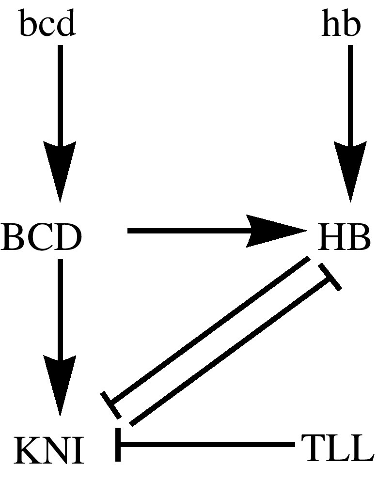
Genetic regulatory network graph associated with the cross regulation of the proteins HB and KNI in Drosophila early development. The protein KNI is activated in the embryo by BCD. HB has a maternal origin and is also regulated by BCD. Both KNI and zygotically produced HB repress each other. In Fig. 2, we show the distribution of HB at the end of the maternal phase, before considering the regulation by BCD as described in this genetic network graph.

In order to test the validity and completeness of the genetic regulatory network in Fig. 4, we took from the FlyEx database the experimental data of the distribution of HB and KNI for the late cleavage cycle 14, and we have integrated numerically in Mathematica the model equations generated by the GeneticNetworks.m software package. The free parameters on the model equations were determined with a bi-objective optimization technique (§ 3.3), minimizing the mean squared deviations between the model solutions and the experimental data (27). Denoting by HB(x, t) and KNI(x, t) the solutions of the model equations, we have fitted the experimental data for the antero-posterior distribution of HB and KNI with the functions α_hbHB(x, t) and α_kniKNI(x, t), where α_hb and α_kni are proportionality constants. The introduction of the proportionality constants α_hb and α_kni is due to the fact that experiments do not correspond to a direct measurement of local protein concentration, but it is proportional to protein concentration. These proportionality constants change from one protein to another. With these two additional proportionality constants and time as a free parameter, we have fitted the 23 parameters of the model with a bi-objective optimization technique and we have calculated the associated Pareto front in the reduced chi-squared space.

In Fig. 5, we show the data for HB and KNI and the corresponding fits. From the fits, it is clearly shown that the genetic regulatory network of Fig. 4 describes well the HB distributions away from the posterior tip of the Drosophila embryo, x < 80. The distribution of the KNI protein is also well described away from the anterior tip of the embryo, x > 20. On the other hand, complementarity of the proteins HB and KNI in the middle region of the embryo is observed. This fact suggests that there are other proteins that regulate the anterior and the posterior regions of the embryo. For the case of regulation of the production of HB in the posterior region of the embryo, a plausible candidate is the Huckebein (HKB) protein, Margolis et al. [12].

Fig. 5
Dots and error bars represent the mean values and the standard deviations of the concentration of the proteins Hunchback (HB) and Knirps (KNI) along the antero-posterior axis of the embryo of Drosophila, at the end of cleavage cycle 14A. The fit has been obtained by a multi-objective optimization technique as described in § 3.3. The continuous lines correspond to the differential equation model solutions α_hbHB(x, t^*) and α_kniKNI(x, t^*), away from the steady state t* < ∞), and for a particular set of parameter values localized on the Pareto front of the bi-objective optimized solution. In this case, the fitted value of time is t^* = 10 s, and the fitted proportionality constants have the values α_hb = 0.1 and α_kni = 2.0. The penalized chi-squared values, (27), of these fits are $χ_{H B}^{2} ({\vec{p}}_{4}) = 0.28$ and $χ_{K N I}^{2} ({\vec{p}}_{4}) = 0.50$ , where p₄ is the vector of the parameters that have been fitted. In this case, P = 23. This fit shows that the genetic regulatory network of Fig. 4 describes well the HB distribution away from the posterior tip of the embryo of Drosophila, x > 80, as well as the distribution of KNI away from the anterior pole of the embryo, x > 20.

In order to analyze the distribution of HB near the posterior region of the embryo, there is experimental evidence that Huckebein (HKB) protein has a band near the posterior pole of the embryo, repressing the zygotic production of HB. Therefore, we introduce HKB in the gap-gene regulatory network as in Fig. 6. As there is experimental evidence that HKB represses the production of HB near the posterior pole of the embryo, we assume a band type localization of HKB near the posterior tip of the embryo.

Fig. 6
Genetic regulatory network graph associated with the cross regulation of the proteins Hunchback (HB), Knirps (KNI) and Huckebein (HKB) in Drosophila early development. The transcription repression of HKB on the transcription of HB is described in Margolis et al. [12].

Following the same steps as in the modeling of the previous section § 2.1, we assume that the HKB protein is localized with the following steady state distribution:

H K B_{e q} (x) = 2 \frac{b_{1}}{e^{2 b_{2} / L} - 1} \cosh (b_{2} \frac{x}{L}) (\sinh (b_{2} \frac{P_{2}}{L}) - \sinh (b_{2} \frac{P_{1}}{L}))

+ \frac{b_{1}}{2} (e^{- b_{2} (x + P_{1}) / L} - e^{- b_{2} (x + P_{2}) / L}) + I_{b c d} (x)

(26)

where P₁, P₂, b₁ and b₂ are constants to be fitted and have the same meaning as the constants in the BCD equilibrium distribution (14). Under these conditions, we have derived with the software package GeneticNetworks.m a new set of equations associated with the graph of interactions of Fig. 6 (Supplementary file S1). We have assumed that HKB is distributed according (26) and, to find the parameter values for the new model, we have done a bi-objective optimization analysis for the new model. As we have a bi-objective optimization problem having as goals the HB and KNI antero-posterior distribution, we have calculated the associated Pareto front in the reduced chi-squared space. In Fig. 7, we show one of the Pareto instances of the fit of the model with the experimental data for HB and KNI. We show also the fitted distribution of the protein HKB.

Fig. 7
Dots and error bars represent the mean values and the standard deviations of the concentration of the proteins Hunchback (HB) and Knirps (KNI) along the antero-posterior axis of the embryo of Drosophila, at the end of cleavage cycle 14A. Due to the lack of experimental data on HKB its spatial experimental distribution is not represented. The fit has been obtained by a bi-objective optimization technique for HB and KNI, having also as free the parameters that describe the HKB distribution (26). The continuous lines correspond to the differential equation model solutions α_hbHB(x, t^*), α_kniKNI(x, t^*) and HKB_eq(x), for a particular set of parameter values localized on the Pareto front of the bi-objective optimized solution. In the case, the fitted value of time is t^* = 29.1 s, and the fitted proportionality constants have the values α_hb = 0.11 and α_kni= 0.65. The penalized chi-squared value, (27), of this fit are $χ_{H B}^{2} ({\vec{p}}_{5}) = 0.14$ and $χ_{K N I}^{2} ({\vec{p}}_{5}) = 0.59$ , where p₅ is the vector of the parameters that have been fitted. In this case, P = 31. The parameter values found for the prediction of the HKB distribution (26) are: P₁ = 0.856, P₂ = 0.873, b₁ = 296.74 and b₂ = 121.87. The HKB distribution found in the fit corroborates the existence of a stripe of the protein HKB near the posterior pole of the embryo as suggested experimentally. This fit supports the statement that the genetic regulatory network of Fig. 6 describes well the distribution of HB along all the antero-posterior axis of the embryo of Drosophila.

The quality of the fits in Figs. 5 and 7 were evaluated from the penalized chi-square functions,

\begin{array}{r} χ_{H B}^{2} (\vec{p}) & = & \frac{1}{n - P / 2} \sum_{i = 1}^{n} \frac{{(H B_{e q} (x_{i}, \vec{p}) - H B_{m e a n} (x_{i}))}^{2}}{H B_{σ^{2}} (x_{i})} \\ χ_{K N I}^{2} (\vec{p}) & = & \frac{1}{n - P / 2} \sum_{i = 1}^{n} \frac{{(K N I_{e q} (x_{i}, \vec{p}) - K N I_{m e a n} (x_{i}))}^{2}}{K N I_{σ^{2}} (x_{i})} \end{array}

(27)

where

\vec{p}

is the vector of the free parameters for the differential equation model and P is the dimension of the vector

\vec{p}

(P = 23 for Fig. 5, and P = 31 for Fig. 7).

From the fits in Fig. 7, we conclude that the transcriptional cross repression of HB over KNI and the transcriptional repression of HKB over HB describe well the spatial distributions of the HB protein along all the antero-posterior axis of the embryo of Drosophila. This result also predicts the approximate distribution of the protein HKB. However, the distribution of the KNI protein is not well fitted in the anterior region x < 20, suggesting the existence of an addition regulation mechanism.

Another important conclusion common to both fits is that gap-gene protein expression is a dynamic process with a very fast expression time, of the order of 30 s (Fig. 7). This expression time is calculated relative to the beginning of cleave stage 14A.

Programs and software tools for multi-objective optimization techniques and Pareto front solutions are available in the Supplementary material [15].

3 Materials and methods

In this section, we briefly describe the algorithms that we have applied to calculate the parameters that best fit the experimental data to the model equations generated by the Mathematica software package GeneticNetworks.m. These algorithms are based on the Covariance Matrix Adaptation Evolution Strategy (CMA-ES) approach, an evolutionary algorithm for black-box continuous optimization [22,23]. The first algorithm is for single-objective optimization, used in § 2.1, and will be referred by CMA-ES. The second algorithm is the multi-objective version of CMA-ES, used in § 2.2, and uses several CMA-ES processes together with a global Pareto-dominance based selection [24]. In a maximization or a minimization problem, there is a fitness function relative to which an optimization is found. In multi-objective optimization problems, there are several fitness functions, and in general when we optimize in order to a fitness function, we are worsening in order to the other fitness function. Pareto optimization is a way of obtaining optimal solutions that, in a certain sense, are not dominated by other solutions.

3.1 Single-objective optimization: CMA-ES

CMA-ES is an evolutionary algorithm that uses a population of μ parents to generate λ offspring, and deterministically selects the best μ of those λ offspring for the next generation. In this contexts of parameter optimization, parents and offsprings refer to points in the high-dimensional space of parameters.

The parameter identification search problem is done as follows: We take a compact subset X of the parameter space S. The number of the parameter to be identified is the dimension of S. Set an initial point p₀ ∈ X ⊂ S and let C = I_n be a covariance matrix, where I_n is the n × n identity matrix. Then, from the multivariate Gaussian distribution with covariance matrix C and mean value p₀, sample λ offsprings. For each offspring or set of parameter values calculate the solution of the model equations and then calculate the fitness function, in our case the, chi-squared distributions (25). From the best μ (< λ) offsprings, according to the fitness function, recalculate a new mean value p₀ and a new (unbiased estimator) covariance matrix C, and repeat the procedure. After several iterations, the best individual ever found is a candidate for the best choice of parameters. For details see Hansen and Ostermeier [22] and Hansen [23]. The parameter values of the maternal protein distributions in Figs. 1–3 have been determined according to this technique.

3.2 Pareto optimization

Pareto optimization is concerned with the finding of the set of optimal trade-offs between conflicting objectives. Namely, Pareto solutions of a multi-objective problem are optimized solutions such that the value of one-objective cannot be improved without degrading the value of at least another objective. Such best compromises are what is called the Pareto set of the multi-objective optimization problem.

Pareto optimization is based on the notion of dominance. Consider a minimization problem with M real valued objective functions f = (f₁, …, f_M) defined on a subset $X \subset ℝ^{n}$ . A solution of the optimization problem $\bar{x} \in X$ is said to dominate another solution x ∈ X, denoted by $\bar{x} ≺ x$ , if,

\begin{array}{l} \forall m & \in & {1, \dots, M} : \\ (f_{m} (\bar{x}) & \leq & f_{m} (x)) \land (\exists m \in {1, \dots, M} : f_{m} (\bar{x}) < f_{m} (x)) . \end{array}

The Pareto set of an optimization problem is the set of non-dominated solutions of a minimization (maximization) problem. More formally,

Pareto set = {x : (x \in X) \land \bar{x} \in X : \bar{x} ≺ x} .

The Pareto front is the image of the Pareto set in the fitness space,

Pareto front = {f (x) : (x \in X) \land \bar{x} \in X : \bar{x} ≺ x} .

The goal of Pareto optimization is to find the Pareto set of optimized parameters and the Pareto front. Therefore, in a multi-objective approach, the natural choice for unbiased parameter estimation is the determination of the Pareto set of a given optimization problem. In this set, all the solutions are optimized solutions. The distributions of the gap-gene proteins HB and KNI in Figs. 5 and 7 correspond to parameter values on a Pareto set of the bi-objective optimization problem. In general, all the solutions on the Pareto set are equally acceptable [8].

3.3 Multi-objective optimization: MO-CMA-ES

The Multi-Objective CMA-ES (MO-CMA-ES) optimization technique is based on the specific CMA-ES algorithm with a random choice of a large number of initial points in the search parameter space [24]. Once defined the multidimensional parameter search space X, we proceed with the multi-objective optimization technique to determine the Pareto set and Pareto front of the two fitting problems of § 2.2. The MO-CMA-ES techniques can be divided in three steps:

1) In the compact search space X, choose randomly μ parents. For each parent, one offspring is generated with the CMA-ES algorithm. Initially, the CMA-ES algorithm is implemented with the identity as covariance matrix.
2) We now rank the best μ individuals from the set of 2μ individuals found previously. For that we use the concept of Pareto dominance. From the 2μ individuals, we select the set of all the non-dominated individuals and we give them rank 1. We apply the same procedure to the remaining individuals and we obtain the rank 2 individuals [25]. This procedure continues until a last rank is reached.
3) In order to rank the individuals within the same rank of non-dominance found previously, we do a second ranking of individuals within each rank. This second order ranking is done according to an hypervolume measure in the objective space [26]. After this new ranking, we retain only the best μ individuals. With this procedure, we obtain an approximation to the Pareto front with an approximately uniform distribution of individuals within each rank. Then, we repeat these three procedures until a good converge to the Pareto front is achieved.

In Fig. 8, we show the Pareto front for the bi-objective optimization problem associated with the parameter identification describing the distribution of HB and KNI as shown in Fig. 5. We show the position of the fit of Fig. 5 (cross) in the Pareto front of Fig. 8. In Fig. 9, we show two other instances (circles) of the fits of HB and KNI proteins on the Pareto front. Comparing the three fits, we conclude that they are all acceptable.

Fig. 8
Pareto front for the fit of HB and KNI proteins of Fig. 5. In this bi-objective optimization problem, the coordinates of the fitness space are the reduced chi-squared functions $χ_{H B}^{2} (\vec{p})$ and $χ_{K N I}^{2} (\vec{p})$ , where the vector of the parameters $\vec{p}$ is a parameterization of the Pareto front. These functions have been calculated as in (25). The cross represents the particular instance of the parameter values of Fig. 5. The circles represent the two other instances of the HB and KNI fits that are shown in Fig. 9.

Fig. 9
Two instances of the fit of HB and KNI in the Pareto front, represented by circles in Fig. 8. In a, we have the best fit for HB and the worst fit for KNI. In b we have the worst fit HB and the best fit for KNI. As it is seen, all these fits are acceptable for parameter calibration and validation of models. The parameter values are listed in the Supplementary file S1.

In Fig. 10, we show the Pareto front for the fit of Fig. 7 and we mark the particular instance of the parameters of Fig. 7 (cross).

Fig. 10
Pareto front for the fit of Hunchback, Knirps and Huckebein proteins of Fig. 7. The cross represents the particular instance of the parameter values of Fig. 7.

In all the cases shown here, we conclude that the experimental data are optimally realized by an infinite set of parameters. This is particularly important in biology in the case of selection pressure affecting simultaneously several phenotypic characteristics of organisms.

4 Conclusions and final remarks

In order to describe the expression of the gap-gene protein Hunchback along the antero-posterior axis of the embryo of Drosophila, we have analyzed a genetic regulatory network model for the proteins HB and KNI and we have calibrated the experimental data with the model predictions. In the most complete version of the model of Fig. 6, we have shown that the distribution of HB along the antero-posterior axis of the embryo are in fact well described by a cross regulation mechanism between HB and KNI together with the transcriptional repression of HKB over HB. We have predicted the distribution of HKB in the form of a localized stripe near the posterior tip of the embryo. This same genetic regulatory network fails to predict the distribution of KNI near the anterior pole of the embryo suggesting the existence of an additional regulation mechanism. In this approach, gap-gene proteins do not diffused along the embryo. Recently [27] obtained a similar prediction of the localization of the HKB protein, additionally regulated by the proteins Giant and Caudal and Krüppel. These authors considered that gap-gene proteins diffuse along the antero-posterior axis of the Drosophila embryo.

Another important conclusion we have obtained is that the antero-posterior patterns of gap-gene proteins are obtained as transient solutions of an ordinary differential equation model, with diffusion playing no role at the level of gap-gene protein expression patterns. With this approach, diffusion is only relevant for the establishment of gradients for proteins produced from mRNA with maternal origin. The patterning obtained along the embryo results from the differences in concentrations of the maternal proteins of the embryo.

The calibration and validation of the genetic regulatory network models have been done with evolutionary algorithm techniques for parameter identification. We have used single-objective and multi-objective techniques within the evolutionary algorithms formalism, and we have analyzed the usefulness of the concept of Pareto optimization in biology. Due to similarities between the fits and the experimental data, it is plausible to think that, in the presence of several objectives, the number of possible parametric solutions of a given problem is not unique, producing an infinite set of parameter instantiations. In this framework, the Pareto set and the Pareto front are the correct approach to analyze these problems. In the case of selection pressure on organisms affecting simultaneously several phenotypic characteristics, the Pareto type solutions appear as the right quantitative approach to quantify phenotypic variability.

In the most difficult case of the multi-objective optimization problem analyzed here, we have fitted 31 parameters in a system of ordinary differential equations with 18 independent variables, and we have implemented these algorithms in a grid computing environment. In the Supplementary material of this paper, we list all the algorithms and all the associated C files developed under this framework [15]. These techniques are general and can be used in other parameter identification problems.

Acknowledgments

This work has been supported by European project GENNETEC, FP6 STREP IST 034952. The parallel computations in this article have been made in the Laboratoire de recherche en informatic of the INRIA, Université Paris-Sud, Paris.

Bibliographie

[1] G. Frigerio; M. Burri; D. Bopp; S. Baumgartner; M. Noll Structure of the segmentation gene paired and the Drosphila PRD gene set as part of a gene network, Cell, Volume 47 (1986), pp. 735-746

[2] W. Driever; C. Nüsslein-Volhard A gradient of bicoid protein in Drosophila embryos, Cell, Volume 54 (1988), pp. 83-93

[3] M. Akam The molecular basis for metameric pattern in the Drosophila embryo, Development, Volume 101 (1987), pp. 1-22

[4] C. Nüsslein-Volhard Gradients that organize embryo development, Scientific American, Volume 275 (1992) no. 2, pp. 54-61

[5] B. Houchmandzadeh; E. Wieschaus; S. Leibler Precise domain specification in the developing Drosophila embryo, Physical Review E, Volume 72 (2005), p. 061920

[6] F. Alves; R. Dilão Modelling segmental patterning in Drosophila: maternal and gap genes, Journal of Theoretical Biology, Volume 241 (2006), pp. 342-359

[7] R. Dilão; D. Muraro mRNA diffusion explains protein gradients in Drosophila early development, Journal of Theoretical Biology, Volume 241 (2010), pp. 342-359

[8] R. Dilão, D. Muraro, M. Nicolau, M. Schoenauer, Validation of a morphogenesis model of Drosophila early development by a multi-objective evolutionary optimization, algorithm, Proceedings of the 7th European Conference on Evolutionary Computation, Machine Learning and Data Mining in BioInformatics, EvoBIO, 2009, Springer Verlag, Tubingen, Germany, April 15–17, 2009.

[9] A. Spirov; K. Fahmy; M. Schneider; E. Frei; M. Nooll; S. Baumgartner Formation of the bicoid morphogen gradient: an mRNA gradient dictates the protein gradient, Development, Volume 136 (2009), pp. 605-614

[10] B.J. Cha; B.S. Koppetsch; W.E. Theurkauf In vivo analysis of Drosophila bicoid mRNA localization reveals a novel microtubule-dependent axis specification pathway, Cell, Volume 106 (2001), pp. 35-46

[11] K.M. Forrest; E.R. Gavis Live imaging of endogenous RNA reveals a diffusion and entrapment mechanism for nanos mRNA localization in Drosophila, Current biology: CB, Volume 13 (2003), pp. 1159-1168

[12] J.S. Margolis; M.L. Borowsky; E. Steingrmsson; C.W. Shim; J.A. Lengyel; J.W. Posakony Posterior stripe expression of hunchbackis driven from two promoters by a common enhancer element, Development, Volume 121 (1995), pp. 3067-3077

[13] E. Poustelnikova; A. Pisarev; M. Blagov; M. Samsonova; J. Reinitz A database for management of gene expression data in situ, Bioinformatics, Volume 20 (2004), pp. 2212-2221

[14] A. Pisarev; E. Poustelnikova; M. Samsonova; J. Reinitz FlyEx, the quantitative atlas on segmentation gene expression at cellular resolution, Nucleic Acids Research, Volume 37 (2009), p. D560-D566

[15] R. Dilão, D. Muraro, Supplementary material for parameter calibration of genetic regulatory, models. https://sd.ist.utl.pt/Download/download.html, 2009.

[16] K. Kozlov; E. Myasnikova; M. Samsonova; J. Reinitz; D. Kosman Method for spatial registration of the expression patterns of Drosophila segmentation genes using wavelets, Computational Technologies, Volume 5 (2000), pp. 112-119

[17] E. Myasnikova; D. Kosman; J. Reinitz; M. Samsonova Spatio-temporal registration of the expression patterns of Drosophila segmentation genes (T. Lengauer; R. Schneider; P. Bork; D. Brutlag; J. Glasgow; H.W. Mewes; R. Zimmer, eds.), Seventh International Conference on Intelligent Systems for Molecular Biology, AAAI Press, Menlo Park, 1999, pp. 195-201

[18] E. Myasnikova; A. Samsonova; K. Kozlov; M. Samsonova; J. Reinitz Registration of the expression patterns of Drosophila segmentation genes by two independent methods, Bioinformatics, Volume 17 (2001) no. 1, pp. 3-12

[19] F. Alves; R. Dilão A simple framework to describe the regulation of gene expression in prokaryotes, C. R. Biologies, Volume 328 (2005), pp. 429-444

[20] R. Dilão; D. Muraro A software tool to model genetic regulatory networks. Applications to the modeling of threshold phenomena and of spatial patterning in Drosophila, PLoS ONE, Volume 5 (2010) no. 5, p. e10743

[21] J. Jaeger; J. Reinitz On the dynamic nature of positional information, BioEssays: news and reviews in molecular, cellular and developmental biology, Volume 28 (2006), pp. 1102-1111

[22] N. Hansen; A. Ostermeier Completely derandomized self-adaptation in evolution strategies, Evolutionary Computation, Volume 9 (2001) no. 2, pp. 159-195

[23] N. Hansen, The CMA evolution strategy: a tutorial. http://www.lri.fr/hansen/cmaesintro.html, 2008.

[24] C. Igel; N. Hansen; S. Roth Covariance matrix adaptation for multi-objective optimization, Evolutionary Computation, Volume 15 (2007) no. 1, pp. 1-28

[25] K. Deb; A. Pratap; S. Agarwal; T. Meyarivan A fast and elitist multiobjective genetic algorithm: NSGA-II, IEEE Transactions on Evolutionary Computation, Volume 6 (2002) no. 2, pp. 182-197

[26] J.D. Knowles, D.W. Corne, M. Fleisher, Bounded archiving using the Lebesgue measure, Proceedings of CEC, vol. 4, IEEE Press, 2003, pp. 2490–2497.

[27] M. Ashyraliyev; K. Siggens; H. Janssens; J. Blom; M. Akam; J. Jaeger Gene circuit analysis of the terminal gap-gene huckebein, PLoS Computational Biology, Volume 5 (2008), p. e1000548

Commentaires - Politique

Ces articles pourraient vous intéresser

Bicoid mRNA diffusion as a mechanism of morphogenesis in Drosophila early development

Rui Dilão

C. R. Biol (2014)

Translational regulation during oogenesis and early development: The cap-poly(A) tail relationship

Federica Piccioni; Vincenzo Zappavigna; Arturo C. Verrotti

C. R. Biol (2005)

Towards a synthetic view of axis specification mechanisms in vertebrates: insights from the dogfish

Marion Coolen; Arnaud Menuet; Sylvie Mazan

C. R. Biol (2009)