Polymer degradation during processing

Xavier Colin; Jacques Verdu

doi:10.1016/j.crci.2006.06.004

Résumés

Anglais
Français

This paper deals with the degradation processes occurring during polymer processing. Some general aspects of polymer processing are first recalled. Then, oxidation mechanisms and kinetics are evoked and the main processing methods are compared from this point of view. Temperature–molar mass maps allow to define a processability window and to envisage ways to widen this window. The final chapter is devoted to a case study: the PET processing, which is characterized by an especially complex combination of degradation processes. .

Cet article traite des processus de dégradation se produisant pendant la mise en forme des polymères. Tout d'abord, certains aspects généraux de la mise en forme des polymères sont rappelés. Ensuite, les mécanismes et la cinétique d'oxydation sont évoqués et les principales méthodes de mise en forme sont comparées de ce point de vue. Les cartes température–masse molaire permettent de définir une fenêtre dans laquelle la mise en forme est possible et d'envisager différentes solutions pour élargir cette fenêtre. Le dernier chapitre est consacré à une étude de cas : la mise en forme du PET, qui est caractérisée par une combinaison spécialement complexe de processus de dégradation. .

1 Introduction

One of the main sources of problems, in polymer processing, comes from the high melt viscosity of the polymers. The consumption of mechanical energy and the cost of tools (for instance injection moulds), could be considerably lowered and the productivity would be increased if the viscosity were decreased by one (or several) order(s) of magnitude. Most of the industrial thermoplastic polymers are processed in the 400–650 K temperature interval. It is clear that processing in the 800–1000 K interval, where viscosities are expected to be typically 10–1000 times lower, would minimize many important technological and economical constraints. Unfortunately, this is impossible, because polymers are thermally instable at these temperatures. Processing operations are always performed in temperature domains where the melt viscosity is relatively high, just below what is called the thermal stability ceiling (TSC). But this latter is a diffuse boundary: there is no discrete threshold for degradation processes. Thus, the optimum processing conditions involve generally a small sacrifice of the structural integrity of macromolecules, as schematized in Fig. 1.

Fig. 1
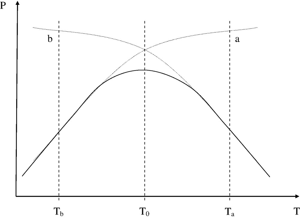
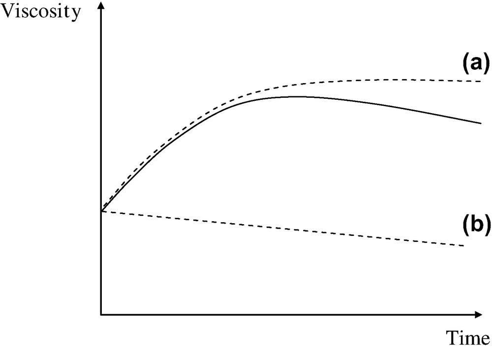
Schematization of the effect of processing temperature (the processing time is supposed constant) on part property.
(a) Effect of physical parameters. (b) Effect of thermal degradation.

At low temperature (T_b), thermal degradation is negligible, but defects due to high melt viscosity are responsible for low part quality.

NB: Mechanochemical degradation processes can also occur in this region.

At high temperature (T_a), the part quality is essentially limited by thermal ageing. Thermal degradation can affect processing properties through, essentially, molecular mass changes, but these effects are generally neglected in process modeling. The corresponding structural changes can however affect the long-term properties (Fig. 2).

Fig. 2
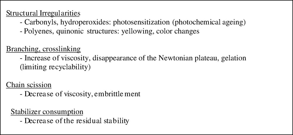
Main types of structural changes during processing, their main consequences.

The aim of this lecture is to try to make a general analysis of polymer degradation processes during processing, starting from the basic principles of polymer physics and degradation kinetics.

NB: Here, the term ‘degradation’ is taken in its widest sense: it covers any process leading to a change of use properties.

Then, the case of PET extrusion will be examined in details to illustrate the complexity of the problem.

2 Thermal ageing during processing. Some general aspects

2.1 Isothermal ageing characteristics

Let us consider a use property P and its threshold value P_F required for the application under consideration. When the polymer undergoes isothermal ageing at the temperature T, P varies and one can define a conversion ratio x for this ageing process:

x = \frac{P_{t} - P_{F}}{P_{0} - P_{F}}

(1)

where P₀ and P_t are the property values at, respectively, the beginning of exposure and after the time t of exposure.

It is thus possible to establish the ageing function at the temperature T:

x = f (t)

(2)

and the lifetime t_F such that:

t_{F} = f^{- 1} (0)

(3)

where f⁻¹ is the reciprocal function of f.

Eq. (3) means that $P = P_{F}$ i.e. $x = 0$ when $t = t_{F}$ .

The lifetime t_F is a decreasing function of temperature (Fig. 3).

Fig. 3
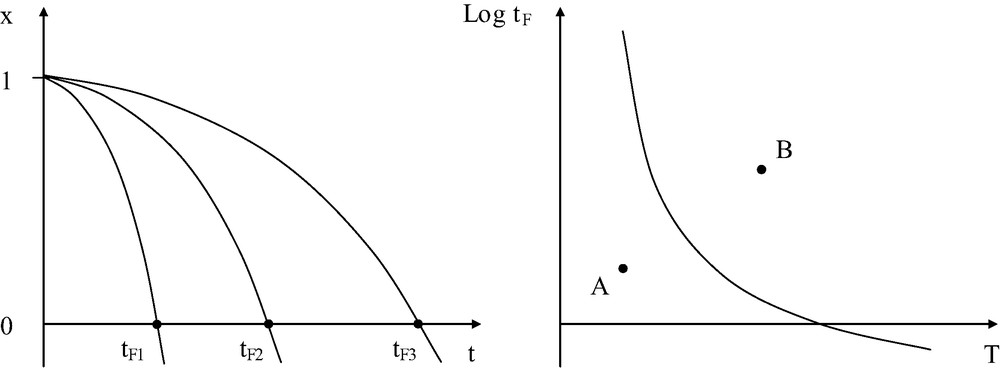
Left: principle of determination of t_F in kinetic degradation curves. Right: shape of the temperature dependence of lifetime.

The history of a given sample, used in given conditions, can be represented by a point in the time–temperature space. Its position relatively to the curve $t_{F} = f (t)$ gives immediately an information on its probable further evolution: if the point (for instance A in Fig. 3 (right)) is below the curve, this means that the material disposes of a residual lifetime. If, in contrast, the point is above the curve (for instance B), this means that the probability of failure is close to unity. Since the 1940s [1], it has been generally assumed that the TSC can be represented by an Arrhenius equation:

t_{F} = t_{F_{0}} exp [\frac{H}{R T}]

(4)

There are, however, many reasons to suppose that Arrhenius equation is, in many cases, inadequate to represent lifetime variations in large temperature intervals. Very powerful models, directly derived from mechanistic schemes and free of simplifying hypotheses, are now available thanks to the existence of efficient numeric computing tools, as shown for instance in the case of radical oxidation of hydrocarbon polymers [2]. Even the problem of polymers stabilized by synergetic combinations of antioxidants is not insuperable [3].

2.2 Non isothermal, static or dynamic ageing

A processing machine can be considered as a chemical reactor displaying non-uniform temperature and shear fields. A first complication appears immediately: degradation occurs in non-isothermal regime. The distribution of residence times in the machine [4], especially the existence of stagnation zones, must be taken into account. Another complication can come from the possible role of shearing. First, it can play a role similar to stirring in (molecular) liquid reactors, favoring thus the homogenization of the reaction medium, that can be important, for instance, in the case of stabilizers with low diffusivity. The difference between ‘static’ (no shear) and ‘dynamic’ thermal ageing are well documented in the literature of the 1960s and 1970s. Shearing can also induce mechanochemical chain scissions of which the main characteristic is to be disfavored by a temperature increase [5]. In the following, it will be considered that ageing tests are performed in conditions representative of processing ones.

Let us now return to the problem of non-isothermal ageing. Our reasoning will be based on the use of graphs in which the polymer history, during a given processing operation, is represented by a single temperature value T_P that can be defined as follows. The process under consideration is characterized by the time t_P during which the polymer stays in liquid state. It is also characterized by the final degradation index x_P of the polymer. T_P is defined as the temperature of an isothermal test that would lead to the degradation index x_P after the exposure time t_P. In other words, T_P is the temperature of isothermal exposure equivalent to the process history for the chosen processing conditions. The determination of T_P can be illustrated by the sample example of zero-order process obeying Arrhenius law:

\frac{d x}{d t} = r; r = r_{0} \exp [- \frac{H}{R T}]; T = f (t)

(5)

So that:

x_{P} = \int_{0}^{t_{W}} r d t = r_{0} \int_{0}^{t_{W}} exp [- \frac{H}{R f (t)}] d t = r_{0} F (t_{W})

(6)

where t_W is the whole processing time and F(t_W) the primitive function of

exp [- \frac{H}{R f (t)}]

According to the chosen definition of T_P:

x_{P} = r_{0} (exp [- \frac{H}{R T_{P}}]) t_{P} i . e . T_{P} = \frac{H}{R l n (F (t_{W}) / t_{P})}

(7)

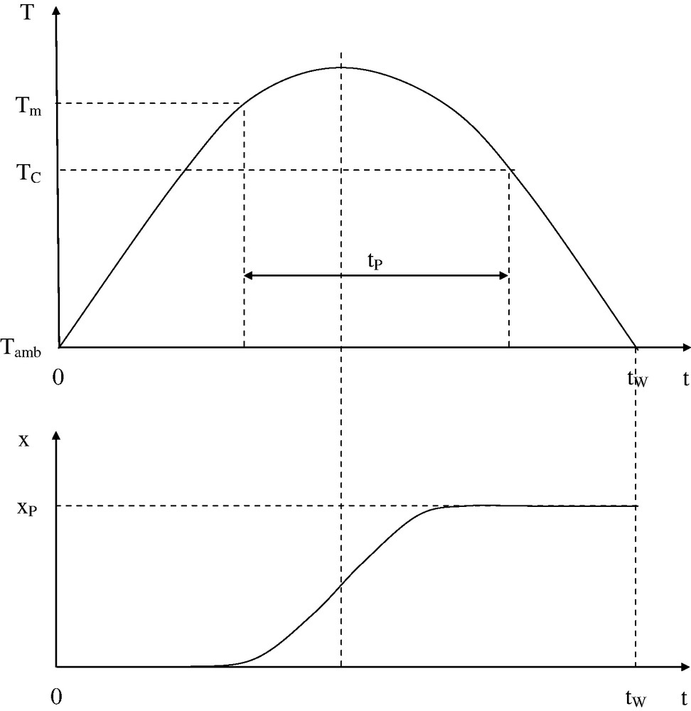
Consider a temperature history $T = f (t)$ for a given processing operation. It is characterized by its whole duration t_W and by the time t_P spent in the liquid state (Fig. 4).

Fig. 4
Above: Temperature history: the whole processing time is the time spent above ambient temperature (T_amb).
t_P is the time elapsed in liquid state (T_m = melting point, T_C = crystallization temperature, for a semi-crystalline polymer. Otherwise, T_m and T_C are replaced by the glass-transition temperature T_g for an amorphous polymer).
T_P is defined as the temperature of an isothermal test that would lead to the same degradation level as the processing operation after an exposure of duration t_P.

2.3 The problem of small conversions of the degradation process

Let us consider three of the main practical consequences of degradation during processing: a change of rheological properties, embrittlement in solid state and color change (for instance yellowing). Rheological property changes can essentially result from molecular weight changes. In the case of random chain scissions, the number n of chain scissions is:

n = \frac{p}{M_{W}} - \frac{p_{0}}{M_{W 0}} = \frac{p_{0}}{M_{W 0}} (\frac{p}{p_{0}} \frac{M_{W 0}}{M_{W}} - 1) = \frac{1}{M_{n 0}} (\frac{p}{p_{0}} \frac{M_{W 0}}{M_{W}} - 1)

where p and p₀ are the polydispersity index values, respectively, after and before ageing.

The Newtonian viscosity change is linked to the molar mass change by a well-known power law:

\frac{η}{η_{0}} = {(\frac{M_{W 0}}{M_{W}})}^{3.4} s o t h a t n = \frac{1}{M_{n 0}} (\frac{p}{p_{0}} {(\frac{η_{0}}{η})}^{0.294} - 1)

At low conversion, p/p₀ is in the order of unity. Thus, the number of chain scission events in order to divide the Newtonian viscosity by a factor 2, for instance, is in the order of:

$n \approx \frac{0.2}{M_{n 0}} i.e. for most of industrial polymers:$

$n \leq 10^{- 2}$ mol kg⁻¹.

Crosslinking affects also rheological properties: gelation occurs when the number of crosslinks becomes equal to the number of weight average chains:

$n \approx \frac{1}{M_{W 0}} i.e. in general:$

$n \leq 2 \times 10^{- 2}$ mol kg⁻¹

Indeed, noticeable changes of the rheological behavior will appear far from the gelation point.

Yellowing results generally from the formation of conjugated polyenes (vinyl polymers) or oxidation products of aromatic rings such as quinones or polyphenols (aromatic polymers). The eye sensitivity to such structural changes depends on many parameters: initial color, presence or not of pigments, mode of sample illumination, sample thickness, etc.

But it is often relatively high, because two characteristics are combined:

● these chromophores have often a high absorptivity, for instance ε > 10⁴ l mol⁻¹ s⁻¹ for most of the above cited species, or a high emissivity when color changes are linked to luminescence as in the case of aromatic species;
● at least for initially white samples, very small spectral changes can be visually detected.

In most of the cases, chromophore concentrations less than 10⁻³ mol kg⁻¹, almost undetectable by IR or NMR, can be the source of noticeable industrial troubles.

Hydroperoxides resulting from thermal oxidation during processing play a key initiating role in further thermal or photochemical ageing in use conditions and can thus significantly affect the material's durability. In the case of thermal oxidation, in the absence of antioxidants, a critical value of the hydroperoxide concentration could be ${[P O O H]}_{C} = k_{1 u} / k_{1 b}$ , where k_1u and k_1b are the respective rate constants of uni- and bimolecular POOH decomposition. In PE, for instance, ${[P O O H]}_{C} = 2.1 \times 10^{- 2}$ mol kg⁻¹ at 500 K [6]. In the presence of antioxidants, for which the usual concentrations are generally in the 10⁻³–10⁻² mol kg⁻¹ range, it is usually assumed that each hydroperoxide decomposition event leads to the consumption of one or two antioxidant molecules.

It can be concluded from this brief survey that relatively small structural changes are sufficient to induce significant variations of use properties such as rheological, mechanical, optical or durability ones. Studies in this field are thus confronted to the analytical difficulties relative to the measurement of small concentrations. It is well known, for instance, that PET hydrolysis cannot be monitored by routine IR or NMR measurements. PP oxidation leads to embrittlement before any detectable change of the IR spectrum, despite the relative high sensitivity of the IR titration of carbonyl groups [7]. In the same way, color can appear in PVC far before structural changes are detectable by IR or NMR.

3 Oxidation

3.1 Mechanistic and kinetic aspects – a brief survey

Oxidation displays two very important features:

● it is a radical chain process propagated by H abstraction:
- ○ (II) P° + O₂ → PO₂° ( $k_{2} \approx 10^{8} - 10^{9}$ l mol⁻¹ s⁻¹ [8]);
- ○ (III) PO₂° + PH → PO₂H + P° ( $k_{3} \approx 1.5 \times 10^{10} exp [- 73000 / R T]$ l mol⁻¹ s⁻¹ for PE [9]).
● the hydroperoxides resulting from propagation are unstable. The dissociation energy of the O–O bond is about 150 kJ mol⁻¹ against more than 250 kJ mol⁻¹ for most of the polymer bonds. The decomposition of hydroperoxides generates radicals:
- ○ (I_u) POOH → PO° + °OH ( $Δ G \approx$ 100 kJ mol⁻¹ at 100 °C);
- ○ (I_b) POOH + POOH → PO° + PO₂° + H₂O ( $Δ G \approx$ 30 kJ mol⁻¹ at 100 °C).

These free-energy values can be compared to the C–C scission one: (I_P) P–P → 2P° ( $Δ G \approx$ 280 kJ mol⁻¹ at 100 °C for a polymethylenic sequence).

All these features explain well the main characteristics of oxidation processes:

● since they are radical chain processes, it is possible to envisage stabilizing ways by reducing the initiation rate or increasing the termination rate;
● the propagation rate depends essentially on the strength of the broken CH bond (Scheme 1).

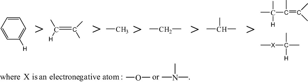
This order corresponds well to the observed hierarchy of polymer stabilities: polymers containing only aromatic or methyl groups (polyimides, polysulfones, polycarbonate, polydimethylsiloxane) are more stable than PE, whereas polymers containing tertiary CH (PP), allylic CH (polydienes) or CH in α of electronegative atoms (PA, POM, etc.) are less stable than PE.
● Due to its ‘closed-loop’ character, oxidation begins at low rate (which allows us to envisage efficient stabilization by antioxidants in low concentration), but displays an autoaccelerated behavior, linked to POOH accumulation.
● In the case of ‘pure’ thermal ageing, hydroperoxide decomposition (I_u or I_b) is expected to largely predominate over polymer decomposition (I_P) at low temperature. The Arrhenius plot of lifetime is expected to have the shape of Fig. 5.
Let us recall that fast and intense shearing can also induce mechanochemical processes, i.e. mechanically activated reactions (I_P) that can participate to the initiation of oxidation radical chains but tend to suppress the ‘closed-loop’ character. Hydroperoxide decomposers such as organic phosphites, which are considered as good processing antioxidants, are not efficient against mechanochemical reactions.
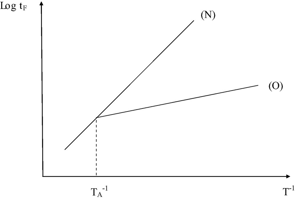
● Let us return to propagation processes (II) and (III). Since $k_{3} < < k_{2}$ , it is easy to see that, in oxygen excess, hydrogen abstraction (III) is the rate-controlling step, whereas, at low oxygen concentration, oxygen addition to radicals (II) becomes the rate-controlling step and the whole oxidation rate becomes sharply dependent on the oxygen concentration.

Fig. 5
Schematization of the shape of the Arrhenius plot for thermal ageing in the presence (O) and in the absence (N) of oxygen.
NB: The dependence is not necessary linear.

In the absence of stabilizer, terminations are expected to be bimolecular:

● (IV) P° + P° → inactive products ( $k_{4} \approx 10^{8} - 10^{12}$ l mol^–1 s⁻¹);
● (V) P° + PO₂° → inactive products ( $k_{5} < k_{4}$ );
● (V) PO₂° + PO₂° → inactive products + O₂ ( $k_{6} < k_{5}$ ).

The effects of oxygen concentration C is summarized in Fig. 6.

Fig. 6
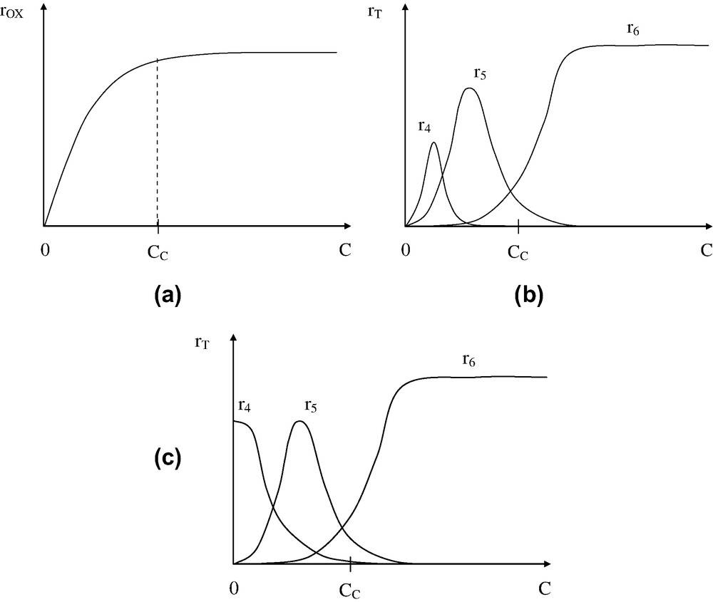
Effect of oxygen concentration C on global oxidation rate (a) and termination rates without (b) and with (c) reaction (I_P).

Two regimes can be thus distinguished:

● regime E (oxygen excess) for $C > C_{C}$ . It is characterized by the fact that oxidation rate is independent of oxygen concentration and reactions involving P° radicals are negligible;
● regime L (low oxygen concentrations) for $C < C_{C}$ . It is characterized by the fact that the oxidation rate is concentration-dependent and reactions involving P° radicals are not negligible.

The limiting (equilibrium) oxygen concentration in the polymer C_S is linked to the oxygen pressure p:

$C_{S} = S p$ , where S is the O₂ solubility, which ranges, for most of the polymers, between 10⁻⁵ and 10⁻⁴ mol m⁻³ Pa⁻¹.

Thus, in air, at atmospheric pressure, C_S takes a value (almost temperature-independent) in the order of 10⁻³ mol l⁻¹. This value is to be compared with the substrate concentration, for instance $[P H] \approx$ 60 mol l⁻¹ in PE, 20 mol l⁻¹ in PP or 14 mol l⁻¹ in PET.

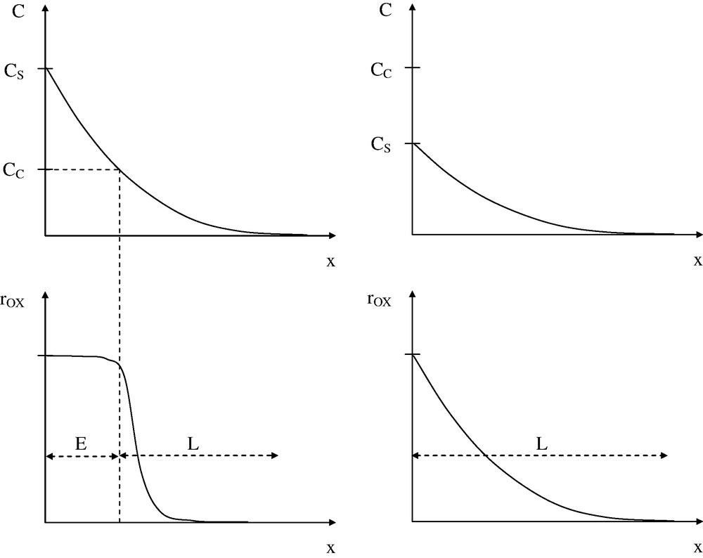
Two polymer families can be distinguished, depending on their behavior in atmospheric air ( $p = 0.02 M P a$ ): those for which $C_{S} > C_{C}$ (for instance PE) [10] and those for which $C_{S} < C_{C}$ (for instance PP) [11]. The regime E will be only observable, in these conditions, for the polymers of the first family and only in thickness layers close to the air–polymer interface since oxidation is expected to be diffusion controlled (Fig. 7).

Fig. 7
Above: oxygen concentration C profile in a bulk sample (x is the depth from the air–polymer interface). Below: profile of oxidation rate (or concentration of oxidation products).
Left: polymer of PE type. Right: polymer of PP type.

Oxidation processes lead generally to a complex mixture of reaction products among which chain scissions (s) and crosslinks (x) are especially interesting for us, because they are susceptible to modify the mechanical and rheological behavior at low conversions.

The most general ‘mechanically active chemical events’ are the following:

● β scissions of alkoxy radicals (Scheme 2). Alkoxy radicals coming from POOH decomposition or from non-terminating PO₂° bimolecular combinations can propagate radical chains by H abstraction, but they can also rearrange by β scission and this latter is often (but not always) a chain scission;
● β scissions of P° radicals (Scheme 3).

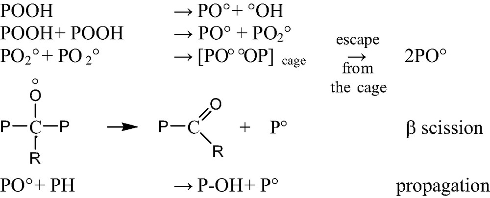
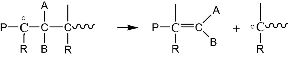
This process is favored in polymers having weak monomer–monomer bonds (PMMA, POM, PP, etc.). It leads to the polymerization radical, which can itself rearrange (depolymerization), abstract hydrogens or terminate;
● coupling of P° radicals:
Both reactions can occur at processing temperatures, disproportionation being favored by a temperature increase.

It is thus possible to distinguish various polymer families as a function of their predominant behavior in regime L: PP, PMMA and POM, for instance, undergo predominant chain scission because alkyl radicals rearrange easily by β scission. In contrast, PE, PET and presumably polymers containing polymethylenic sequences undergo predominant crosslinking because P° radicals react mostly by coupling. PVC, in which the weakest bond is C–Cl, is a particular case owing to the importance of HCl zip elimination processes and the probable occurrence of crosslinking reactions involving conjugated polyenes. Since these latter are easily oxidizable, one can distinguish regime E (low color, predominant chain scission) from regime L (high color, predominant crosslinking).

3.2 Stabilization against oxidation

There are many excellent books and reviews on polymer thermal stabilization [12]. An exhaustive review of the main stabilization ways would be out of the scope of this lecture. Here, we will focus only on the main antioxidant families (not specific of the polymer structure), e.g. radical-chain breaking antioxidants (phenols, amines) and hydroperoxide decomposers (sulfides, phosphites).

The chain breaking antioxidants scavenge PO₂° radicals. Their stabilization mechanism can be schematically represented by an unique reaction competitive to H abstraction:

● (III) PO₂° + PH → POOH + P° (k₃) ;
● (S) PO₂° + InH → POOH + Q (k_S);

where Q is a species unable to propagate the radical chain.

The efficiency of the stabilizer can be linked, in a first approach, to the rate ratio:

λ_{S} = \frac{r_{S}}{r_{3}} = \frac{k_{S} [I n H]}{k_{3} [P H]}

λ_S must be in the order of unity (or higher) for an efficient stabilizer. Since, for economical and technical reasons:

\frac{[I n H]}{[P H]} \leq 10^{- 3} .

This means that, to be efficient, a stabilizer must be characterized typically by:

\frac{k_{S}}{k_{3}} \geq 10^{3}

But k_S and k₃ have distinct activation energies, for instance in PE: $E_{S} \leq 20 kJ m o l^{- 1}$ [13] and $E_{3} \approx 73 kJ m o l^{- 1}$ [9]. In other words, $k_{S} / k_{3}$ is a decreasing function of temperature. These stabilizers are thus expected to be generally less efficient in the processing than in the used-temperature range.

The hydroperoxide decomposers destroy hydroperoxides by non-radical mechanisms:

(D) POOH + Dec → inactive products (k_D).

This reaction is competitive with the initiation one, for instance, for a predominant unimolecular POOH decomposition:

(I_u) POOH → 2P° (k_1u).

Here also, the stabilizer is expected to be efficient if the rate ratio is in the order of unity or higher:

\frac{r_{D}}{r_{1 u}} = \frac{k_{D} [D e c]}{k_{1 u}} \geq 1

Unfortunately, there are no literature data, to our knowledge, on activation energies of k_D. What is well known by practitioners is that sulfides are appropriate to use (low-temperature) conditions, whereas phosphites are rather appropriate to processing conditions [12].

There are also extensive reviews on transport properties of antioxidants, at least in polyolefin matrices [14]. But most of the published data concerns solid-state properties. Both the solubility S and the diffusivity D are increasing functions of the temperature but for both quantities, the Arrhenius parameters, compiled from literature, display a compensation effect [15], with a compensation temperature always close to 80–100 °C. We have thus the following alternative:

● this effect is a reality. In this case, the hierarchy of solubility and diffusivity values at high temperature (in the molten state) would be opposite to low temperature (solid-state) one. Such behavior would be paradoxical: it is difficult to imagine, for instance, that the diffusivity of molecules increases with their size;
● we are in presence of an artifact, linked, for instance, to the non-Arrhenian temperature dependences of S and D. This hypothesis, which seems more reasonable than the preceding ones, suggests that the determination of transport properties of additives in molten-state polymers is a totally open research problem, needing probably novel experimental approaches.

3.3 Oxidation in processing conditions

As far as oxidation is concerned, a given processing operation is mainly characterized by two main factors: the residence time t_P, as defined in Section 1.1, and the mode of polymer oxygenation. The main processing operations can be schematically described by Table 1.

Operation	Polymer state	Processing time	Oxygenation	Additive loss
Injection molding	Liquid	Short (≈ 1 min)	Limited	Disfavored
Extrusion	Liquid	Short (a few minutes)	Limited	Disfavored
Calendaring	Liquid	Medium	Full	Favored
Rotomoulding	Liquid	Long	Full	Favored
Thermoforming	Solid (rubbery)	Short	Full	Disfavored
Welding	Liquid	Short	Full	Disfavored

In the case of extrusion and injection molding, the polymer is almost totally confined; oxygenation is limited to the polymer–air interface in the feeder zone. Antioxidant loss by evaporation is disfavored, except possibly in the case of film-extrusion blowing. The profile of oxygen concentration is expected to have the shape of Fig. 8.

Fig. 8
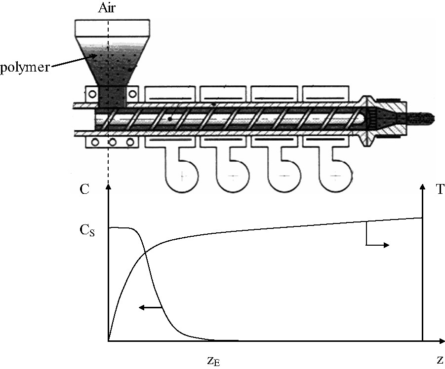
Schematization of the oxygen concentration C and temperature profiles in the case of extrusion or injection molding.

The depth z_E of the oxygenated zone will depend on three variables: oxygen diffusivity in the melt, rate of polymer transport in the machine and temperature profile (i.e. rate of oxygen consumption). Indeed, this partial confinement favors clearly the regime L.

Calendaring and, especially, rotomoulding are characterized by the length of the stage during which the hot (liquid) polymer is exposed to air (several dozens of minutes in the case of rotomoulding, which is, no doubt, the most critical process from the point of view of polymer degradation). Thermoforming is expected to be less ‘degrading’, owing to the relatively low maximum temperature. In contrast, degradation at noticeable extent can be observed in certain cases of welding (by hot air streams) were the shortness of the hot stage cannot compensate the (sometimes very high) maximum temperature.

4 Polymer processability

4.1 Temperature–molar mass maps

A given processing method is characterized by an optimal viscosity range corresponding to melt-flow index values ranging from less than 0.1 (pipe extrusion) to more than 10 (paper coating). Schematically, the melt flow index is proportional to the reciprocal of the viscosity, this latter being a sharply increasing function of the molar mass (at low shear rates: $M F I = K M_{W}^{- 3.4}$ where K is an increasing function of the temperature). It appears thus convenient to study the processability conditions in temperature–molar mass maps. Two important boundaries can be defined in this map:

● the solid-rubbery/liquid boundary, i.e. the glass-transition temperature (T_g) for amorphous polymers or the melting temperature (T_m) for semi-crystalline polymers. Both temperatures are increasing functions of the molar mass in the low molar mass range (where M_C is the entanglement threshold whose structure–property relationships are relatively well known [16]). T_g continues to increase with M_n above M_C according to the Fox–Flory law:

T_{g} = T_{g ∞} - \frac{K_{F F}}{M_{n}}

where K_FF is in the order of 10–100 K kg mol⁻¹, so that T_g tends to be almost independent of molar mass when this latter is higher than 10–100 kg mol⁻¹. K_FF is an increasing function of T_{g_∞} (which depends essentially on the chain stiffness).
T_m tends to decrease very slowly with the chain length far above M_C because entanglements tend to perturb crystallization;
● the rubber–liquid boundary T_L, which can be more or less arbitrarily defined as the end of the rubbery plateau, the G′–G″ crossover (G′ and G″ being the components of the complex shear modulus), the terminal relaxation time [17], etc. For us, this boundary can be defined as follows: the viscosity, for a given shear rate γ^o, can be expressed as the product of two functions:

η = f (T) g (M)

Let us consider the high viscosity limit for the process under consideration:

η_{max} = f (T_{L}) g (M)

one obtains:

f (T_{L}) = \frac{g (M)}{η_{max}} and T_{L} = f^{- 1} (\frac{g (M)}{η_{max}}) = F (M)

Thus, for a given molar mass M, this function represents the boundary $T_{L} = F (M)$ such that for $T < T_{L}$ , the polymer would have a viscosity too high to be processable, whereas for $T > T_{L}$ , it would be, in principle, processable. In the case of a Newtonian viscosity obeying to Arrhenius law, one would have (for $M_{W} > M_{C}$ ):

η_{m a x} = K_{0} (exp [\frac{H_{V}}{R T}]) M_{W}^{3.4} i .e . T_{L} = \frac{H_{V}}{R ln \frac{η_{max}}{K_{0} M_{W}^{3.4}}}

The temperature–molar mass map would thus have the shape of Fig. 9.

Fig. 9
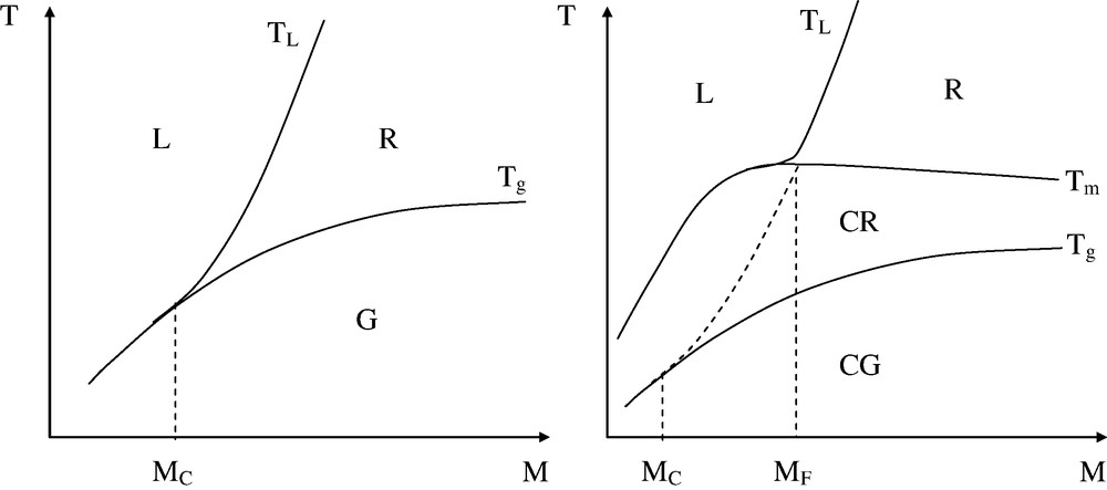
Shape of the temperature–molar mass maps (logarithmic scale for M) for an amorphous polymer (left) and a semi-crystalline polymer (right).
G: glassy domain; R: rubbery domain; L: liquid domain; CG: semi-crystalline polymer with the amorphous phase in glassy state; CR: semi-crystalline polymer with the amorphous phase in rubbery state.

In all the cases, there is a critical molar mass M_C corresponding to the onset of the entanglement regime. Schematically, for an amorphous polymer:

T_{L} \approx T_{g} for M \leq M_{C}

and

T_{L} > T_{g}

for

M \geq M_{C}

(T_{L} - T_{g})

is an increasing function of M.

For a semi-crystalline polymer, there is a molar value M_F higher than M_C such that:

T_{L} \approx T_{m} for M \leq M_{F}

and T_{L} \geq T_{m} for M \geq M_{F}

M_F is the molar mass of the polymer for which the length of the rubbery plateau corresponds to the distance between T_m and T_g.

Most of the thermoplastic processing operations (except thermoforming or machining) involve at least one elementary step in liquid state, i.e. above T_L, but, indeed, thermal degradation limits accessible temperature range.

4.2 The TSC

The temperature at the degradation threshold can be defined from the quantities and relationships established in Section 1.2. If x_F is the endlife criterion for the conversion ratio of the degradation process, it is possible to define an ‘equivalent isothermal temperature’ T_D such that: for $T_{P} = T_{D}$ , $x_{P} = x_{D}$ .

In other words, degradation would just reach the endlife criterion at the end of the processing operation if $T_{P} = T_{D}$ . According to Eqs. (5)–(7):

F (t_{W}) = \frac{x_{D}}{r_{0}}

so that

T_{P} = \frac{H}{R l n (x_{D} / r_{0} t_{P})}

4.3 The brittle limit

All the polymers are brittle when their molar mass is lower than a critical value M′_C. In most of the cases (amorphous polymers and semi-crystalline polymers except apolar ones), M′_C $\approx (2 - 3) M_{C}$ [18]. Ductility and toughness are essentially linked to the existence of an entanglement network.

In apolar polymers (PE, PP, PTFE), M′_C $\approx (20 - 30) M_{C}$ [19]. This peculiarity seems to be linked to the specific role of the chains interconnecting crystallites.

This critical molar mass value constitutes an important vertical boundary in the temperature–molar mass maps: polymers are easily processable below M′_C, but they cannot be used, in practice, owing to their very high brittleness. Typically, M′_C is in the order of 10–20 kg mol⁻¹ for many usual amorphous (PC) or semi-crystalline (PET, PA11, etc.) polymers and in the order of 100–200 kg mol⁻¹ for PE, PP or PTFE.

4.4 The processability window

It is then possible to build the temperature–molar mass map for a given polymer. It must have, in the most common cases, the shape of Fig. 10.

Fig. 10
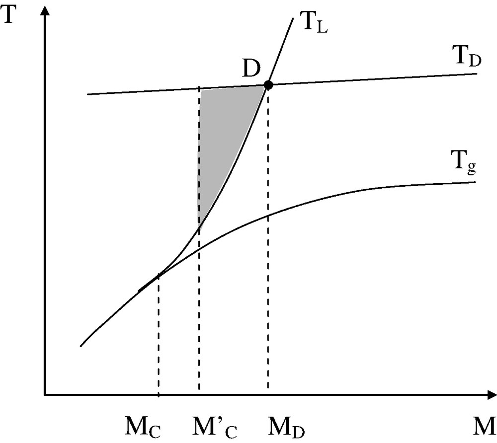
Temperature–molar mass map. The dashed zone corresponds to the processability window.

Let us consider the intersection point D between the thermal degradation ceiling T_D and the ‘rheological threshold’ T_L. It corresponds to a molar mass M_D that can be defined as follows: for $M > M_{D}$ , processing (for the given temperature–time history) is impossible because the material cannot be maintained in liquid state for the desired time without a catastrophic thermal degradation. Each polymer is thus characterized by a molar mass interval M′_C–M_D in which the processing operation under consideration can be used to obtain parts having acceptable use properties.

4.5 Usual ways to widen the processability window

The processability window appears as a trigonal domain of which one boundary: M′_C is a material property that cannot, in principle, be shifted. There are thus two ways to widen the processability window, corresponding to the two remaining boundaries (see Fig. 11).

Fig. 11
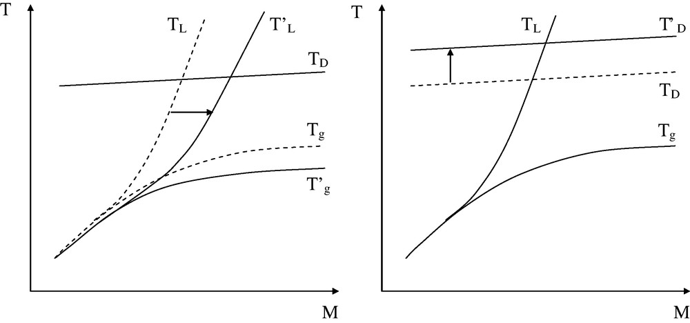
Shifting the boundaries of the processing window by modifications of the composition. Left: use of processing aids (plasticizers, lubricants, etc.). Right: use of thermal stabilizers. The dashed line corresponds to the starting polymer and the arrow indicates the sense of the modification.

There are cases where the TSC of the unstabilized polymer is so low as M_D < M′_C. In other words, there is no way to process this polymer in the entangled regime (see Fig. 12).

Fig. 12
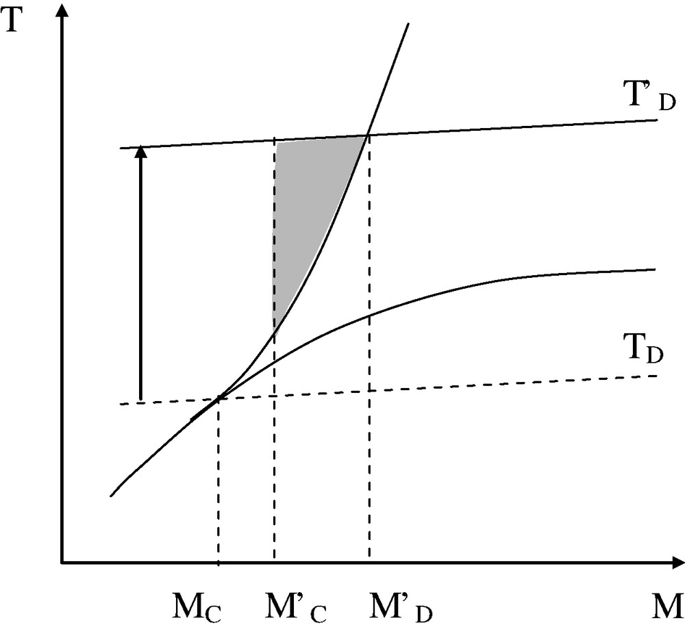
Case of unprocessable unstabilized polymers: in the absence of stabilization (T_D), M_D < M′_C, there is no way to obtain a ductile/tough polymer by the processing method. With a stabilizer (T′_D), M_D is shifted above M′_C, there is a processability window (dashed area).

PVC and PP, for instance, belong to this family of materials: there is no way to process these polymers without an efficient system of stabilization, which explains the amount of literature on their thermal stabilization. PVC is a very interesting but complicated case because in this polymer, certain stabilizers, for instance metal soaps, can act as lubricants, whereas others, for instance alkyltin thioglycolates, display a non-negligible plasticizing effect. A complete understanding of these stabilization processes needs, no doubt, the detailed knowledge of both chemical and physical aspects. An interesting peculiarity of PP, is its very high critical molar mass M′_C $\approx$ 200 kg mol⁻¹: embrittlement can occur at an extremely low conversion of the oxidation process, practically undetectable by chemical or spectrochemical titrations [20]. This characteristic can explain the relative sensitivity of this polymer to recycling. Indeed, in the (very frequent) case where the polymer perishes by oxidation, it is possible to envisage a significant widening of the processability window by inerting the zones of polymer oxidation especially by nitrogen. This effect could be schematized by Figs. 11 (left) or 12, in which T_D is the thermal degradation ceiling in air, whereas T'_D is the TSC in neutral atmosphere.

5 A case study: PET processing

5.1 PET characteristics

PET is a semi-crystalline polymer with a melting point at $T_{m} \approx$ 255 °C. Indeed, the processing temperature cannot be lower than T_m. It is usually close to 280 °C. The embrittlement molar mass of PET M′_C is close to 15 kg mol⁻¹. Since, for industrial grades, the initial molar mass is not higher than ≈ 60 kg mol⁻¹, this means that the number of chain scissions to reach embrittlement is such that:

$s \leq \frac{1}{15} - \frac{1}{60} =$ 0.05 mol kg⁻¹, a value to be compared, for instance, to the monomer concentration [m] = 5.2 mol kg⁻¹.

PET displays two very important features: the existence of ester groups extremely reactive with water at 280 °C and the existence of a dimethylene sequence highly reactive with oxygen at this temperature. Thus, three main processes are expected to occur in the temperature range of extrusion/injection:

● the hydrolysis/polycondensation process;
● the anaerobic thermal degradation process;
● the oxidation process.

5.2 Hydrolysis–condensation

The mechanism can be written as follows:

E+W ⇌_{k_{R}}^{k_{R}} Al+Ac

where E is the ester group, W is the water molecule, Al and Ac the chain end alcoholic and acid groups resulting from hydrolysis. These latter are supposed to be in equal concentrations:

{[A l]}_{0} = {[A c]}_{0} = {[A]}_{0}

in the initial state (before processing).

Hydrolysis is expected to predominate if the initial water concentration is higher than the equilibrium concentration:

{[W]}_{∞} = \frac{k_{R}}{k_{H}} \frac{{[A]}_{0}^{2}}{{[E]}_{0}}

The number of chain scissions at equilibrium is thus:

s_{∞} = {[W]}_{0} - {[W]}_{∞} = {[W]}_{0} - \frac{k_{R}}{k_{H}} \frac{{[A]}_{0}^{2}}{{[E]}_{0}}

In fact, in polyesters, $k_{R} / k_{H}$ is relatively low and $A_{0}^{2} / E_{0} \approx 10^{- 4}$ so that $s_{∞} \approx {[W]}_{0}$ . The number of chain scissions is almost equal to the initial number of water molecules. In other words, [W]₀ must be significantly lower than 0.05 mol kg⁻¹, e.g., 900 ppm, to avoid embrittlement. All these characteristics are well known by practitioners: PET granules must be carefully dried prior to processing. On the other hand, heating in dry state (with ${[W]}_{0} < {[W]}_{∞}$ , thus favoring polycondensation), allows us to restore high molar mass values in hydrolytically degraded samples [21]. The effects of the hydrolysis–condensation process on the polymer structure can be considered reversible in the long term since one has always the possibility to ‘repair’ the chain scissions. Indeed, they can be also catastrophic in the short term if the initial water concentration is in the order of 900 ppm, e.g., less than 10 times lower than the equilibrium concentration in the amorphous phase at ambient temperature.

5.3 Anaerobic thermal degradation

Transesterification is expected to occur at high temperature in PET. It can modify the molar mass distribution until an equilibrium distribution is reached. It can also generate macrocycles as observed by MALDI TOF experiments [22]. But, in the absence of oxygen, PET degrades essentially by a non-radical mechanism involving a rearrangement of the ethylene ester (Scheme 4).

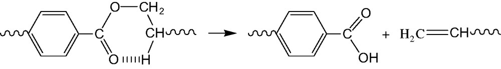
This process has been investigated by many authors [23]. It can be considered, in a first approach, irreversible. It is very slow in usual processing conditions and predominates only in the long term when the hydrolysis–condensation process has reached its equilibrium (see Fig. 13).

Fig. 13
Shape of melt viscosity changes during an isothermal exposure at 280 °C in dry state. The curve displays a maximum linked to the existence of two components (dashed lines): the polycondensation (a) and the thermal degradation (b).

Let us return to the effects of the hydrolysis–condensation phenomenon: the equilibrium molar mass is:

M_{n ∞} = \frac{1}{b_{0} + a_{∞}}

where a_∞ is the equilibrium acid (or alcohol) concentration:

a_{∞} = {(\frac{k_{H}}{k_{R}} E_{∞} W_{∞})}^{1 / 2} (see preceding section)

and b₀ is the half-concentration of non-condensable chain ends.

The above described thermal degradation process would thus lead to an increase of b₀ in a pseudo-zero-order process:

b_{0} = b_{∞} + r_{T} t

where r_T is the rate of chain scission for this mechanism.

In the frame of a single processing operation, this process is expected to have unsignificant consequences. But the corresponding structural defects accumulate irreversibly, contrarily to hydrolysis ones. Thus, after N recycling operations, one could reach $b_{0} > 1 / 15$ mol kg⁻¹. Then, the molar mass would be lower than M′_C, even in dry equilibrium state, and the polymer would be permanently brittle.

PET chains can also contain weak structures, for instance diethylene oxide groups, which degrade more easily than normal esters. They can be responsible for a fast but limited degradation step, obeying to first-order kinetics:

b_{1} = b_{10} exp - (K_{1} t)

where K₁ is the first-order rate constant for this process.

5.4 Oxidation

According to well-established structure–property relationships, oxidation is expected to attack preferentially the methylene groups in PET. The reactivity of these latter can be more or less influenced by the ester groups to which they are linked, but globally, it is not very different from the reactivity of methylenes in PE, the main difference being essentially in the substrate concentration four to five times lower in PET than in PE. A very important characteristic of PE is that oxidation leads to a predominant chain scission at high oxygen concentrations and to crosslinking at low oxygen concentrations. Both regimes necessarily coexist in the case of PET extrusion or injection molding as a result of oxygen concentration gradients characteristic of these processes, as schematized in Fig. 8. Their existence has been demonstrated from rheometric experiments, as illustrated by the example of Fig. 14.

Fig. 14
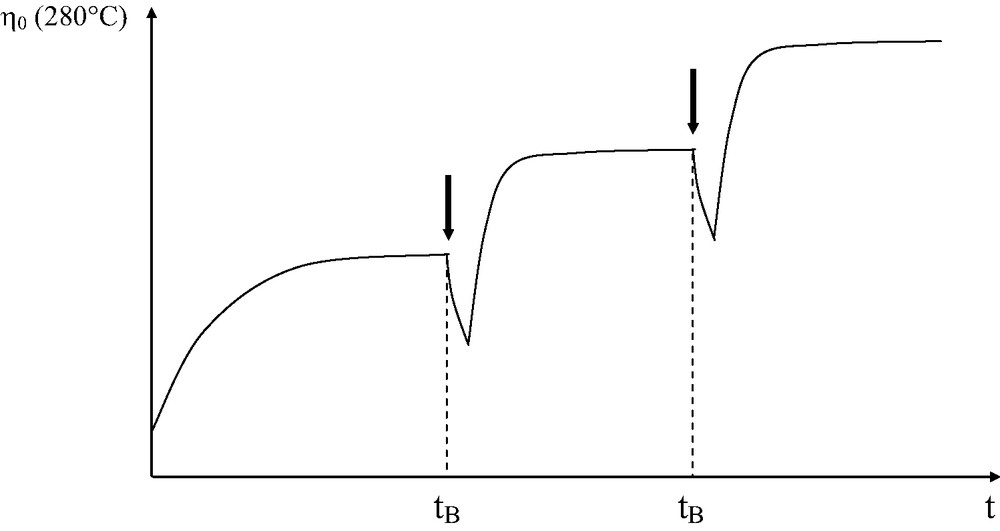
Newtonian viscosity of PET at 280 °C in neutral atmosphere. Air is admitted during a short duration at times t_A and t_B. The viscosity decreases partly as a result of oxidation in oxygen excess. It reincreases when oxygen is almost totally consumed and becomes higher than its initial value as a result of crosslinking. This latter phenomenon can be also detected by the increase of the imaginary component η″ of the complex viscosity η*: before crosslinking, η* = η′; after crosslinking, η* > η′ (η′* = (η′² + i η″²)^1/2).

Finally, oxidative ageing during extrusion is expected to lead to the following structures.

● Propagation PO₂° + PH → POOH + P° (k₃).
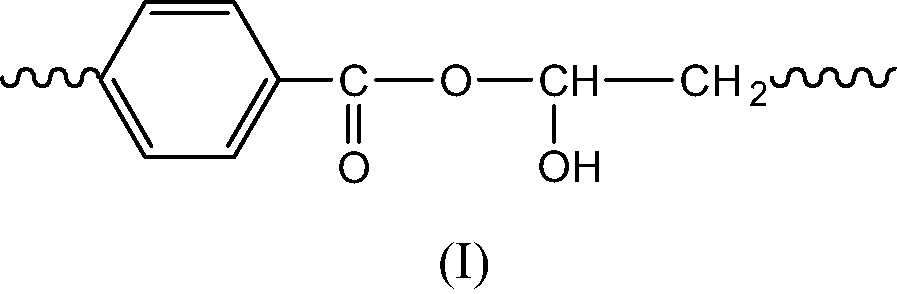
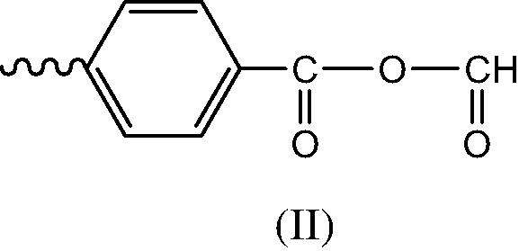
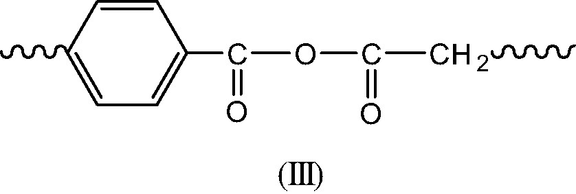
Hydroperoxide groups resulting from propagation events are very unstable at 280 °C, where their decomposition first-order rate constant is expected to be in the order of $k_{1} \approx 4.1 \times 10^{- 2}$ s⁻¹. Their stationary concentration will be thus very low.
● Initiation products. Since POOH decomposition generates PO° radicals, the latter are expected to abstract hydrogens to give the alcohol (I) or to undergo β scission to give the chain end anhydride (II) (Schemes 5 et 6).

● Termination in regions of oxygen excess is expected to give caged PO° radicals leading essentially to the alcohol (I) and the corresponding anhydride (III) (Scheme 7).

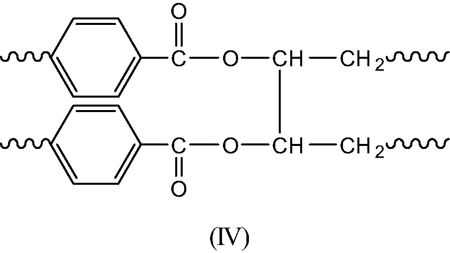
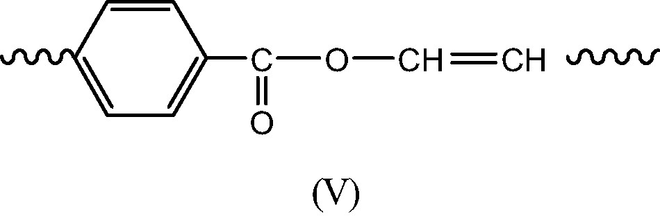
Termination in regions of low oxygen concentration is expected to give essentially long branches (IV) and double bonds (V) resulting of disproportionation of P° radicals (Schemes 8 et 9).

Indeed, some of these structures are relatively reactive at 280 °C: anhydrides are highly sensitive to hydrolysis and they can possibly react in transesterification processes, leading thus to an excess of acid groups. The latter can possibly condensate with tertiary alcohols (I) to give branching. But, branching is expected to result essentially from terminations of P° radicals, a rare event. Thus, in usual extrusion conditions, where polymer oxygenation is disfavored, structural changes will be relatively limited and will not affect, in the short term, the use properties. But, what happens in the long term, after several recycling operations? Long branches are expected to accumulate in the polymer, modifying thus its rheological and mechanical behavior. They accumulate, indeed, very slowly, but they can modify significantly the polymer properties, since one can recall that the branch concentration at the gel point is $\approx M_{W 0}^{- 1}$ , i.e. a very low value.

6 Conclusion

Processing in liquid state cannot be considered, rigorously speaking, as a purely physical operation, because the optimum processing conditions are generally just below the TSC of the polymer. A processability window can be defined in temperature–molar mass graphs. It is limited by three boundaries: the ductile–brittle critical molar mass M′_C, the TSC T_D and a minimum fluidity temperature T_L sharply dependent on the molar mass. Processing aids and thermal stabilizers can shift these boundaries and open the processability window.

When thermal stability is defined on the basis of mechanical (change of rheological properties, embrittlement in the solid state) or optical (color changes) criteria, the TSC corresponds to very low conversions of the degradation processes, that can carry strong analytical problems.

Oxidation lowers always the TSC. It leads to distinguish between processing methods in which the polymer is well oxygenated (for instance rotomoulding) and those where oxygenation is restricted to the feeder zone (extrusion, injection molding). But, even in these latter cases, it cannot be neglected a priori. An important and general characteristic of extrusion is that it can lead to chain scissions at high oxygen concentrations and crosslinking at low oxygen concentrations. Chain scission can lead to embrittlement. Branching can modify seriously the rheological behavior and become catastrophic when it reaches the gel point (which occurs at low conversions, especially for high molar mass polymers). Fortunately, efficient inhibitors exist for polymer oxidation.

The case of PET extrusion illustrates the complexity of structural changes occurring during processing since the following processes occur simultaneously:

● hydrolysis and condensation (the predominating process depends on the water content);
● transesterification, cycle formation;
● thermal degradation by ethylene ester rearrangement;
● thermal degradation by decomposition of weak points (diethylene glycol);
● chain scission resulting of oxidation at high oxygen concentration;
● crosslinking resulting of oxidation at low oxygen concentration.

Oxidation and hydrolysis can predominate in the feeder region, whereas all the other thermal processes are expected to predominate in the zones far from the feeder where oxygen and water are not present, because they have been consumed in the upper part of the machine.

Modeling the polymer degradation during processing needs first a kinetic scheme for degradation processes in isothermal conditions with the corresponding elementary rate constants and their activation energy, and second a model for the history of a polymer particle within the processing machine, taking into account the distribution of residence times, temperature gradients, oxygen concentration gradients, etc. Such models have been elaborated for reactive processing and could be probably adapted to degradation with minor modifications to take into account oxygen transport.